3

I'm a bit confused about applying the FEM using piecewise linear functions.

I think I get understand how to use linear functions. We use the hat function for each element and the solution is $$u_h(x) = \sum_{j=0}^M u_j \phi_j(x) $$ where $\phi_j(x)$ is the hat function for each element and the $u_j$ are obtained by solving a matrix system $Au=f$ where $A$ is the stiffness matrix and $f$ is the load vector.

Now for the problem I have, I am given a 1d quadratic reference element on $[-1,1]$ with nodes $\xi_1 = -1, \xi_2=0$ and $\xi_3$ and shape functions $$\psi_1(\xi) = \frac{1}{2}\xi(\xi-1),\;\;\;\psi_2(\xi) = (1+\xi)(1-\xi),\;\;\;\psi_3(\xi) = \frac{1}{2}\xi(\xi+1). $$ which satisfy $\psi_p(\xi_q)=\delta_{pq}$ for $p,q\in\{1,2,3\}$. Then we are given local and global nodes and other stuff.

I have solved parts of the question where I had to transform each element to use the reference element but am missing the bigger picture. The part I don't understand is about these quadratic reference elements. Why do I have 3 functions now instead of 1 from the linear case? and what is the solution given by now after I solve the equation for the stiffness matrix and load vector because I have 3 functions?

Any help on understand this would be greatly appreciated. Thanks a lot.

Han de Bruijn
  • 17,070
videlity
  • 908
  • I suppose $\xi_3 = +1$ ? Your shape functions are correct then. In the linear case, you have 2 functions instead of 1: $(1-\xi)$ and $(1+\xi)$ if your element is at $[-1,+1]$. It would help if you tell us more about your problem. And about how the connectivity of your elements is defined. Using an element which is not linear can be quite tricky. – Han de Bruijn Nov 02 '13 at 11:28
  • Your approach sounds like a mixture of a finite difference and a finite element method. You could add a tag "finite-elements". But .. now I see it's not in their standard list. – Han de Bruijn Nov 02 '13 at 11:44
  • for a given mesh $0=x_0<x_1<x_2<\ldots<x_M=r$ we have local nodes $z_{kp} = \frac{1}{2}[(1-\xi_p)x_{k-1}+(1+\xi_p)x_k],1\leq k\leq M, 1\leq p\leq 3, $ and global nodes $z_{2k} = x_k$ for $0\leq k\leq M$ and $z_{2k-1} = \frac{1}{2}(x_{k-1}+x_k).$ the shape functions for $k$th element $[x_{k-1},x_k]$, $$\psi_{kp}(x)=\psi_p(\xi) \qquad \text{where } x=\frac{1}{2}[(1-\xi)x_{k-1}+(1+\xi)x_k]$$ which satisfy $\psi_{kp}(z_{kq}) = \delta_{pq}$. I found the $M\times 3$ connectivity matrix $C$ such that $z_{kp}=z_j$ iff $j=C_{kp}$ which $[0 1 2; 2 3 4; 4 5 6; ...]$.Im just a bit confused how it all fits – videlity Nov 02 '13 at 11:58
  • Sorry. In my first comment the shape functions should have been $(1-\xi)/2$ and $(1+\xi)/2$ – Han de Bruijn Nov 02 '13 at 11:59
  • so what is the $\phi_j(x)$ in the quadratic case? – videlity Nov 02 '13 at 12:36
  • Couldn't resist so I've posted another answer. Hope you appreciate. – Han de Bruijn Dec 18 '17 at 21:06

3 Answers3

2

This question doesn't have anything to do with finite difference methods, but you probably got the attention of the right people anyway. I think you're missing the idea that you actually have 2 functions in the linear case, not just 1. The "hat function" is really something that arises when you plot the basis functions globally. These are derived from a similar reference element as well though:

Given a 1d linear reference element on $[-1, 1]$, and nodes $\xi_1 = -1, \xi_2 = +1$, with shape functions:

$$ \psi_1(\xi)=-\frac{1}{2}(\xi-1) \quad \psi_2(\xi)=\frac{1}{2}(\xi+1) $$

This set of functions also satisfies the "partition of unity" requirement, just like the quadratic shape functions. The hat functions $\phi_j$ are really just these shape functions mapped from the reference element to the problem domain.

The only change when you go from linear to quadratic elements is that you now are using 3 nodal values and 3 shape functions to interpolate solutions over the rest of the element rather than 2 of each.

Interpolating solutions is exactly the same once you realize this.

1) Locate the element that contains $x$

2) Find the value of $\xi$ corresponding to the value of $x$ within that element

3) Interpolate using the shape functions:

$$ u(x)=\sum_{i=1}^N u_i \psi_i(\xi) $$

where $N$ is the number of nodes in the element and $i$ is the local, not global, index number.

In practice, it is difficult (and unnecessary) to obtain analytical forms of the shape functions in global coordinates, especially when you move to higher dimensions. For this reason, when people say "shape function", they are almost invariably referring to the shape function in the reference element coordinates, so you don't really need a $\phi(x)$ function like you were thinking.

  • Second that. And think it is desirable to add a tag "finite-elements" to the standard tags, but how can this be accomplished? – Han de Bruijn Nov 08 '13 at 20:00
1

Any function $f$ at your quadratic element is interpolated with finite element shape functions, where $(1,2,3)$ are the the nodes (three of them, from the left to the right): $$f(\xi) = \frac{1}{2}\xi(\xi-1) f_1 + (1-\xi^2)f_2 + \frac{1}{2}\xi(\xi+1) f_3$$ This is equivalent with a finite difference representation: $$f(\xi) = f_2 + \frac{1}{2}(f_3 - f_1) \xi + \frac{1}{2}(f_3 - 2 f_2 + f_1) \xi^2$$ Where discretizations of the zero'th, first and second derivative are recognized. Your local nodes obey the same equations, due to isoparametrics: $$z = z_2 + \frac{1}{2}(z_3 - z_1) \xi + \frac{1}{2}(z_3 - 2 z_2 + z_1) \xi^2$$ Therefore if $\,z_2 = (z_1 + z_3)/2$ , as you say, then $z_3 - 2 z_2 + z_1 = 0$. With other words: the quadratic term simply drops out and what we finally have is the same linear element as before.
Due to isoparametrics, the same is valid for any $\,f$, resulting in: $$f_2 = \frac{f_1 + f_3}{2} \quad ; \quad f(\xi) = f_2 + \frac{1}{2}(f_3 - f_1) \xi = \frac{1}{2}(1-\xi) f_1 + \frac{1}{2}(1+\xi) f_3$$ So it's my theory that, e.g. with an equidistant grid, quadratic elements aren't useful. But I have a personal bias towards linear elements, admittedly :-)

Han de Bruijn
  • 17,070
  • Thanks for the help. I'm still a bit confused as to what the solution $u_h$ would be in terms of the quadratic elements :( – videlity Nov 03 '13 at 01:57
0

The one-dimensional Finite Difference stencil / quadratic parent Finite Element is defined geometrically by:

enter image description hereenter image description here

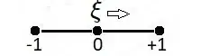
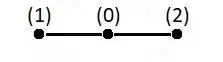
  • three nodal points in local $\xi$-coordinates at $(-1,0,+1)$ , nodes numbered as $(1,0,2)$
  • Algebraically, for any (Test) function $\,T(\xi)$ , it is defined by a quadratic interpolation, part of a Taylor series expansion: $$ T = T(0) + \frac{\partial T}{\partial \xi}(0).\xi + \frac{1}{2} \frac{\partial^2 T}{\partial \xi^2}(0).\xi^2 $$ Because of the mapping $(T_1,T_0,T_2) \to (-1,0,+1)$ it follows that: $$ T_0 = T(0)\\ T_1 = T(0) - \frac{\partial T}{\partial \xi}(0) + \frac{1}{2} \frac{\partial^2 T}{\partial \xi^2}(0)\\ T_2 = T(0) + \frac{\partial T}{\partial \xi}(0) + \frac{1}{2} \frac{\partial^2 T}{\partial \xi^2}(0)\\ \quad \mbox{ F.E. } \leftarrow \mbox{ F.D. } $$ Solving these equations is not much of a problem and well-known Finite Difference schemes are recognized: $$ T(0) = T_0 \\ \frac{\partial T}{\partial \xi}(0) = \frac{T_2-T_1}{2}\\ \frac{\partial^2 T}{\partial \xi^2}(0) = T_1-2T_0+T_2 \\ \quad \mbox{ F.D. } \leftarrow \mbox{ F.E. } $$ Finite Element shape functions may be constructed as follows: $$ T = N_0.T_0 + N_1.T_1 + N_2.T_2 = \\ T_0 + \frac{T_2-T_1}{2}\xi + \frac{T_1-2T_0+T_2}{2}\xi^2 =\\ (1-\xi^2)T_0 + \frac{1}{2}(-\xi+\xi^2)T_1 + \frac{1}{2}(+\xi+\xi^2)T_2 \\ \Longrightarrow \quad \begin{cases} N_0 = 1-\xi^2 \\ N_1 = (-\xi+\xi^2)/2\\ N_2 = (+\xi+\xi^2)/2 \end{cases} $$ Isoparametric means that the same interpolation will be employed for any other function at the element. The global one-dimensional Cartesian coordinate $\,x\,$ itself may serve as an outstanding example of such another function: $$ x = x(0) + \frac{\partial x}{\partial \xi}(0).\xi + \frac{1}{2} \frac{\partial^2 x}{\partial \xi^2}(0).\xi^2\\ x = x_0 + \frac{x_2-x_1}{2}.\xi + \frac{1}{2} (x_1-2x_0+x_2).\xi^2\\ x = (1-\xi^2)x_0 + (-\frac{1}{2}\xi+\frac{1}{2}\xi^2).x_1 + (+\frac{1}{2}\xi+\frac{1}{2}\xi^2).x_2 $$ 
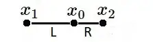
Before trying to establish the inverse transformation - which means solving for $\,\xi$ - we make some substitutions. First assume that $\,x_1 < x_0 < x_2$ ; then define Left arm $\,L = x_0 - x_1\,$ and Right arm $\,R = x_2-x_0\,$ of the element:

    enter image description here
    Algebraically: $$ x = x_0 + \frac{x_2-x_1}{2}.\xi + \frac{1}{2} (x_1-2x_0+x_2).\xi^2 \\ \Longrightarrow \quad \frac{R-L}{2}\xi^2 + \frac{R+L}{2}\xi + x_0 = x \\ \Longrightarrow \quad x(\xi) = \frac{R-L}{2}\left[\xi + \frac{R+L}{2(R-L)}\right]^2 - \frac{R+L}{8(R-L)} + x_0 $$ This means that the curve $\,x(\xi)\,$ is a parabola for $\,R\ne L\,$ and linear for $\,R=L\,$ . Let's assume in the sequel that our element is not the important special case, which is linear.
    If $\,R\ne L$ , then the parabola $\,x(\xi)\,$ is convex and has a minimum for $\,R > L$ , is concave and and has a maximum for $\,R < L$ . A few numerical experiments shall reveal what's going on.
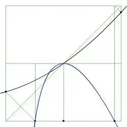
    In the pictures below the viewport is $\,[-1,+1]\times[0,2]$ . Curve in black is the function $\,x(\xi)\,$ with $\,x_0=1$ , curve in $\color{blue}{blue}$ is an isoparametric Test function $\,T(\xi) = 1-\xi^2\,$ with $\,x_0=0$ . Thin lines in $\color{green}{green}$ are for support of the ideas. Regular behavior without any anomalies is displayed first, for $\,R < L$ , $R \approx L$ , $R > L$ :
    enter image description here
    enter image description hereenter image description here
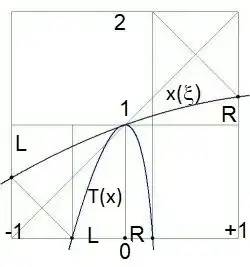
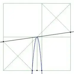
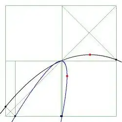
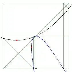
    $\color{red}{Red}$ dots indicate anomalous behavior. Resulting in a Test function which is multi-valued outside the element, ipse est (i.e.): not a function at all. It is seen in the pictures that such is the case if the maximum or minimum of the parabola $\,x(\xi)\,$ is inside the parent element $[-1,+1]$ domain:
    enter image description hereenter image description here
    Therefore, to avoid anomalous behavior, the position of the extreme of the parabola must be outside the $[-1,+1]$ range of the parent element: $$ -\frac{R+L}{2(R-L)} < -1 \quad \mbox{and} \quad -\frac{R+L}{2(R-L)} > +1 $$ Written otherwise: $$ -\frac{R+L}{2(R-L)} + 1 < 0 \quad \Longleftrightarrow \quad \frac{R-3L}{2(R-L)} < 0 \quad \Longleftrightarrow \quad \frac{R/L-3}{2(R/L-1)} < 0 \\ -\frac{R+L}{2(R-L)} - 1 > 0 \quad \Longleftrightarrow \quad \frac{-3R+L}{2(R-L)} > 0 \quad \Longleftrightarrow \quad \frac{L/R-3}{2(L/R-1)} < 0 $$ Thus we only have to solve for the first inequality and then exchange $\,L \leftrightarrow R$ . Here goes: $$ R/L - 1 < 0 \quad \Longrightarrow \quad R/L-3 > 0 \quad \Longrightarrow \quad \begin{cases} R/L > 3 \\ R/L < 1 \end{cases} \quad \mbox{: impossible} $$ But there is another possibility, though only one: $$ R/L - 1 > 0 \quad \Longrightarrow \quad R/L-3 < 0 \quad \Longrightarrow \quad \begin{cases} R/L < 3 \\ R/L > 1 \end{cases} $$ At last, in view of the above, with $\,L \leftrightarrow R$ : $$ \begin{cases} L/R < 3 \\ L/R > 1 \end{cases} \quad \mbox{and} \quad \begin{cases} R/L < 3 \\ R/L > 1 \end{cases} \quad \Longrightarrow \quad \begin{cases} 1/3 < R/L < 3 \\ R/L \ne 1 \end{cases} $$ It is concluded that the one-dimensional quadratic finite element is useful if and only if the quotient of the two arms lengths is between rather narrow boundaries. It must be not to far from linear, so to speak: $$ \frac{\mbox{long arm}}{\mbox{short arm}} < 3 $$ Otherwise you run the risk of having spurious behaviour, which may be even worse - and more difficult to trace - in two or three dimensions. That's one reason why I am definitely in favour of linear instead of higher order (say quadratic) elements.

    Note. Anomalous behavior of the kind is also observed in 2-D, e.g. with quadrilateral elements having an obtuse angle or being self-intersecting. See : Quadrilateral Finite Elements must be convex and not self-intersecting. But why? .

    Sad remark. A detailed analysis as the one above requires little more than some simple algebra and elementary geometry. Yet such an analysis is seldom seen in Finite Element contexts; though the conclusions of such an analysis seem to be important enough. So one can only guess for the reasons why it is not done.

    Han de Bruijn
    • 17,070