Linear system
Given the matrix $\mathbf{A}\in\mathbb{C}^{m\times n}_{\rho}$, and data vector $b\in\mathbb{C}^{m}$, the linear system
$$
\mathbf{A} x = b
$$
will have a least squares solution provide that $b\notin\color{red}{\mathcal{N}\left(\mathbf{A}^{*}\right)}$.
Least squares solution
The least squares solution is defined as
$$
x_{LS} = \left\{
x \in \mathbb{C}^{n} \colon
\lVert
\mathbf{A} x - b
\rVert_{2}^{2}
\text{ is minimized}
\right\}
\tag{1}
$$
As you noted, the least squares solution can be written as
$$
x_{LS} = \color{blue}{\mathbf{A}^{+} b} +
\color{red}{\left(
\mathbf{I}_{n} - \mathbf{A}^{+} \mathbf{A}
\right) y}, \quad y\in\mathbb{C}^{n}
\tag{2}
$$
Fundamental projector
The right hand component is the fundamental projector onto the $\color{red}{null}$ space $\color{red}{\mathcal{N}\left(\mathbf{A}\right)}$
$$
\mathbf{P}_{\color{red}{\mathcal{N}\left(\mathbf{A}\right)}}
=
\color{red}{\left(
\mathbf{I}_{n} - \mathbf{A}^{+} \mathbf{A}
\right)}
$$
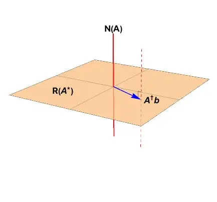
The least squares solution is the affine space represented by the $\color{red}{red}$, dashed lined. The projector projects vectors onto this $\color{red}{null}$ space. (Note the solution of minimum norm is $\color{blue}{x_{+}} = \color{blue}{\mathbf{A}^{+}b}$.)
Full column rank
When the matrix $\mathbb{A}$ has full column rank, $\rho = n$,
the null space $\color{red}{\mathcal{N}\left( \mathbf{A} \right)} = \mathbf{0}$
$\mathbf{P}_{\color{red}{\mathcal{N}\left(\mathbf{A}\right)}}
\color{red}{\left(
\mathbf{I}_{n} - \mathbf{A}^{+} \mathbf{A}
\right)} =
\left(
\mathbf{I}_{n} - \mathbf{I}_{n}
\right) = \mathbf{0}$
least squares solution is the point
$
\color{blue}{x_{+}} = \color{blue}{\mathbf{A}^{+}b},
$
This is the point in the range space $\color{blue}{\mathcal{R}\left(\mathbf{A}^{*}\right)}$
Read more
A bit more background is in Singular value decomposition proof.
Toy problem
$$
\begin{align}
%
\mathbf{A} x &= b \\
%
\left[ \begin{array}{cc}
1 & 0 \\ 0 & 0
\end{array} \right]
%
\left[ \begin{array}{c}
x_{1} \\ x_{2}
\end{array} \right]
%
&=
\left[ \begin{array}{c}
b_{1} \\ b_{2}
\end{array} \right]
\end{align}
$$
If $b_{1}\ne0$, the least squares solution exists. Another way to state this condition is
$$
b\notin\color{red}{\mathcal{N}\left( \mathbf{A}^{*}\right)}
$$
For $b_{2}\ne0$, the general least squares solution can be written as
$$
x_{LS} =
\color{blue}{\left[ \begin{array}{c}
b_{1} \\ 0
\end{array} \right]}
+ \alpha
\color{red}{\left[ \begin{array}{c}
0 \\ 1
\end{array} \right]}, \quad \alpha \in \mathbb{C}
$$
The fundamental projector onto the null space $\color{red}{\mathcal{N}\left(\mathbf{A}\right)}$ is
$$
\mathbf{P}_{\color{red}{\mathcal{N}\left(\mathbf{A}\right)}}
=
\color{red}{\left[ \begin{array}{cc}
0 & 0 \\ 0 & 1
\end{array} \right]}
$$
When $b_{2}=0$, the data vector $b$ is in the $\color{blue}{range}$ space $\color{blue}{\mathcal{R}\left(\mathbf{A}\right)}$, and there is a direct solution
$$
x = \color{blue}{x_{LS}} =
\color{blue}{\left[ \begin{array}{c}
b_{1} \\ 0
\end{array} \right]}
$$
The direct solution is the least squares solution which is a point in the range space.
