Least squares solution
Start with data set $m=5$ points,
$$\left\{ x_{k}, y_{k} \right\}_{k=1}^{m}$$
Model function
$$
y(x) = a x^{b} - c.
$$
Define least squares solution:
$$
(a,b,c)_{LS} = \left\{
(a,b,c) \in \mathbb{C}^{3} \colon
\sum_{k=1}^{m}
\left( y_{k} - a x_{k}^{b} - c \right)^{2}
\text{ is minimized}
\right\}
$$
Compute least squares solution:
$$
\begin{align}
a_{LS} &= 0.6947372490916177, \\
b_{LS} &= 3.6934462148212246, \\
c_{LS} &= 100.57131353798891.
\end{align}
$$
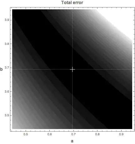
Total error:
$$
r^{2} \left( a_{LS}, b_{LS}, c_{LS} \right) = \sum_{k=1}^{m}
\left( y_{k} - a_{LS} x_{k}^{b_{LS}} - c_{LS} \right)^{2}
= 0.694737
$$
The total error function $r^{2}\left( a, b, c_{LS} \right)$ is plotted below, with the white dot showing the least squares solution.
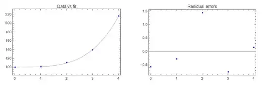
The data points, the predictions, and the residual errors are listed and plotted below. The total error is
$$r^{2} = 3.06477$$.
$$
\begin{array}{crll}
x_{k} & y_{k} & \phantom{w}y(x_{k}) & \phantom{www}r_{k}\\\hline
0 & 100 & 100.571 & -0.571314 \\
1 & 101 & 101.266 & -0.266051 \\
2 & 111 & 109.559 & \phantom{-}1.44078 \\
3 & 140 & 140.754 & -0.754306 \\
4 & 217 & 216.849 & \phantom{-}0.150893 \\
\end{array}
$$
Logarithmic transformation
Logarithmic transformations distort the problem. The solution that follows is not the solution of the original problem (For example, Least Square Approximation for Exponential Functions). This will be more clear when we compare the total errors.
The problem to solve
$$
\begin{align}
y - c = ax^{b}
\end{align}
$$
is replaced with this problem
$$
\begin{align}
\ln (y - c) &= \ln \left(ax^{b}\right) \\
&= \ln a + b \ln x
\end{align}
$$
The logarithmic transformation is an exact map when there is no error. But the fact we resort to least squares is an admission of existence of error. So the transformation only works in the case where we don't use it.
The input data is
\begin{array}{ll}
x & y \\\hline
0 & 0 \\
\ln (2) & \ln (11) \\
\ln (3) & \ln (40) \\
\ln (4) & \ln (117) \\
\end{array}
The outputs are
$$
\ln a = 0.0031410142182181078 \qquad \Rightarrow \qquad a = 1.0031459523722948,
$$
and
$$
b = 3.4097548950738794.
$$
Total error for the transformed problem is
$$
r^{2} = 19.956
$$
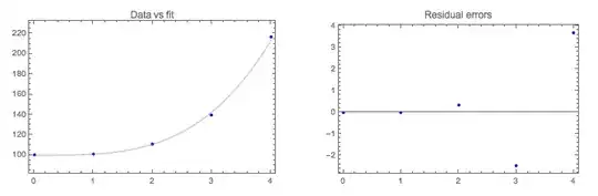
The data, predictions and residual errors are tabulated and plotted below.
$$
\begin{array}{crll}
x_{k} & y_{k}\phantom{w} & \phantom{w}y(x_{k}) & \phantom{www}r_{k}\\\hline
0. & 100. & 100. & \phantom{-}0. \\
1. & 101. & 101.003 & -0.00314595 \\
2. & 111. & 110.661 & \phantom{-}0.338885 \\
3. & 140. & 142.485 & -2.48451 \\
4. & 217. & 213.303 & \phantom{-}3.69707 \\
\end{array}
$$
Note the larger size of the residuals compared to the original fit.
The doubling value in part (d) is found by solving
$$
ax^{b} = 100 \qquad \Rightarrow \qquad
x= 3.85614
$$


