Least Square Approximation for Exponential Functions

Question

I'm a little confused on how to approach the following problem.

Use the least square method to fit a curve of the form $y=a\cdot b^x$ to a collection of $n$ data points $(x_1,y_1),...,(x_n,y_n)$ Find $a$ and $b$.

From what I understand. Given data {$(x_1,y_1),...,(x_n,y_n)$}, we may define the error associated to $y=a\cdot b^x$ by \begin{equation} E(c,d)=\sum_{i=1}^{n}(y_i-a\cdot b^{x_i})^2 \end{equation} The goal is to find values of $a$ and $b$ that minimize the error. In multivariable calculus we learn that this requires us to find the values of $(a,b)$ such that

\begin{array} d \frac{\partial E}{\partial a}=0 & & \frac{\partial E}{\partial b}=0 \end{array}

Differentiating $E(a,b)$ yields:

\begin{eqnarray} \frac{\partial E}{\partial a}&=&\sum_{i=1}^n2(y_i-a\cdot b^{x_i})(-b^{x_i})=0\\ \frac{\partial E}{\partial b}&=&\sum_{i=1}^n2(y_i-a\cdot b^{x_i})(-a\cdot b^{x_i-1}x_i)=0\\ \end{eqnarray}

I know that the least square method tries to minimize the error, but I can't help but feel that I doing this somewhat wrong since this isn't a polynomial - but an exponential - function.

The alternative was for me to take the natural log of $y=a\cdot b^x$ to get: \begin{equation} \ln{y}=\ln{a}+x\ln{b} \end{equation} Then defining $\ln{y}=Y$,$\ln{a}=A$ and $\ln{b}=B$ to get: \begin{equation} Y=A+xB \end{equation} Then from here apply the least square method to my new linear equation.

Any suggestions or feedback on what I can do to solve this problem?

---

Thank you for your time.

Answer 1

The standard approach to solving this question is indeed to linearize by taking the logarithm. The same trick is used for the power law, $y=a\cdot x^b$, among others. This is probably the approach expected by your professor.

Anyway this is a twist as the nonlinear transform does not provide the true minimum solution of the original problem, as the errors themselves are rescaled non-uniformly.

Your formulation is indeed the correct one, but you end-up with a nasty system of equations that has no analytical solution.

So you must resort to a numerical approach such as that of Levenberg and Marquardt which solves these nonlinear equations iteratively. This method requires a good initial approximation, for which one will naturally chose the solution obtained from linearization.

Answer 2

You are perfectly correct making the problem linear. But this only gives you estimates of parameters $a$ and $b$.

Using those, you have to perform a nonlinear regression since what is measured is $y_i$ and not $\log(y_i)$. The first steps minimizes $$\sum_{i=1}^n \big(A+Bx_i-\log(y_i)\big)^2$$ while you need, as you wrote, to minimize $$E=\sum_{i=1}^n \big(a b^{x_i}-y_i\big)^2$$ So, $A,B$ (given by the linear regression) provide estimates of $a,b$ from which you can start the minimization.

Since the estimates would probably be good, you also could use Newton-Raphson method to solve $$\frac{\partial E}{\partial a}=\frac{\partial E}{\partial b}=0$$ with numerical derivatives. For sure, if you have an optimizer, the problem is simple (as Yves Daoust mentioned).

Answer 3

@Claude Leibovici yet again makes a sound argument with solid exposition by pointing out that the linear regression of the logarithmically transformed data does not provide the true solution. He then suggests a Newton-Raphson approach to find the least squares parameters. Another perspective follows which uses least squares to reduce the dimension on the problem and provides an example with solution as demonstration. The difference between the original solution and the solution after the logarithmic transform is amplified.

Original problem A logarithmic transformation creates a problem with a different solution, and should be avoided. The original trial function is $$ y(x) = a b^{x} $$ The input data are the set of points $(x_{k}, y{k})_{k=1}^{m}$. By definition, the method of the least squares minimizes the sum of the squares of the residual errors: $$ \left[ \begin{array}{c} a \\ b \end{array} \right]_{LS} = \left\{ \left[ \begin{array}{c} a \\ b\end{array} \right] \in \mathbb{R}^{2} \bigg | \sum_{k=1}^{m} \left(y_{k} - a b^{x_{k}}\right)^2 \text{ is minimized } \right\} $$ As long as the data contains noise, the transformed equation must have a different solution.

Logarithmic transform A logarithmic transformation yields the trial function $\ln y = \ln a + x \ln b.$ The least squares solution to this problem is $$ \left[ \begin{array}{c} a \\ b \end{array} \right]_{T} = \left\{ \left[ \begin{array}{c} a \\ b\end{array} \right] \in \mathbb{R}^{2} \bigg | \sum_{k=1}^{m} \left(\ln y_{k} - \ln a -x_{k} \ln b \right)^2 \text{ is minimized } \right\} $$ The new problem has a distinct solution.

The logarithm doesn't measure residual error uniformly and the least squares fit is defeated in its attempt to balance errors. The preferred property is a linear transform, such as converting centigrade to Fahrenheit. A difference of 3 degrees transforms to the same value whether the thermometer reads 1 or 100 degrees. Certainly $\ln 4 - \ln 1 \ne \ln 103 - \ln 100$.

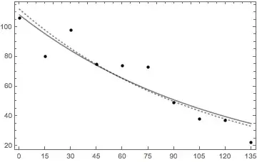
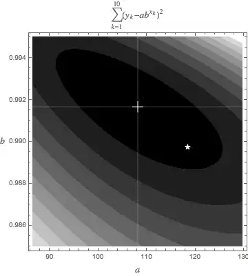
Example To provide an example and a sense of scale, consider a problem from Data Reduction and Error Analysis, 1e, by Philip Bevington, table 6-2, representing measurement for radioactive decay: $$ \begin{array}{rr} time & count\\\hline 0 & 106 \\ 15 & 80 \\ 30 & 98 \\ 45 & 75 \\ 60 & 74 \\ 75 & 73 \\ 90 & 49 \\ 105 & 38 \\ 120 & 37 \\ 135 & 22 \\ \end{array} $$ The least squares solution is $\left[ \begin{array}{c} a \\ b \end{array} \right]_{LS}=\left[ \begin{array}{c} 108.132 \\ 0.99167 \end{array} \right]$ with a $r^{2}\left( \left[ \begin{array}{c} a \\ b \end{array} \right]_{LS} \right)=966$, the minimum value.

If the data are transformed logarithmically, $\left[ \begin{array}{c} a \\ b \end{array} \right]_{T} = \left[ \begin{array}{c} 118.502 \\ 0.9897197 \end{array} \right]$. The value of $r^{2}$ at this point is 1256.

The two solutions are displayed in the plot below show the merit function $r^{2}\left( \left[ \begin{array}{c} a \\ b \end{array} \right] \right)$ using the original trial function. The least squares solution is the central cross at the minimum; the solution for the logarithmically transformed equations is marked by a star.

The following figure plots the different solutions against the data points (solid: original problem, dashed: transformed problem. The previous plot is much more useful for distinguishing between solutions.

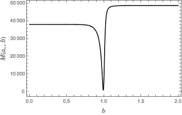
Back to least squares There are many ways to find the minimum of this two dimensional surface. But even better, we can reduce the problem to one dimension. Least squares does offer a path to reduce a two parameter minimization problem to that of one parameter which is easier to solve. Start with the minimization criterion for the linear parameter $a$ $$ \frac{\partial} {\partial a} r^{2} = \sum_{k=1}^{m} \left( y_{k} - a b^{x_{k}}\right)^2 = 0. $$ We can recast this relationship to express $a$ as a function of $b$, $\hat{a}$. This provides a formulation for the best value of $a$ at each value of $b$: $$ \hat{a}(b) = \frac{y_{k}b^{x_{k}}} {b^{2x_{k}}} $$ The merit function is reduced to that of a single variable $$ r^{2}\left( \left[ \begin{array}{c} \hat{a}(b) \\ b \end{array} \right] \right) = r^{2}\left( b \right) = \sum_{k=1}^{m} \left( y_{k} - \frac{y_{k}b^{x_{k}}} {b^{2x_{k}}} b^{x_{k}}\right)^2, $$ a function with a distinct minimum as seen in the following plot.