Magnitudes of components don't tell the full story. It is also about which way they are pointing in comparison to which direction the "neighbor vectors" are pointing and how their magnitudes/directions change.
Consider your example fields plotted as vectors starting from each point.
First the vector field $\vec{f}$:
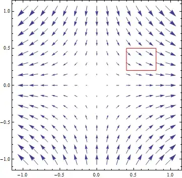
You see that the "flow" goes towards the $x$-axis (because the $j$-component is negative above the $x$-axes and positive below $x$-axis. Also similarly the flow goes away from $y$-axis. More to the point. If you look at a small region there is as much flow entering the region as leaving it = divergence vanishes.
For example if we look at a small region somewhere in the first quadrant (red rectangle in the figure), then there is a little bit more stuff flowing in from the top than what's exiting from the bottom (the $j$ component decreasing), but the difference is exactly compensate by left-to-right components. A little bit more is exiting from the right border than what is entering through the left border.
On the other hand the vector field $\vec{g}$ looks like the following:
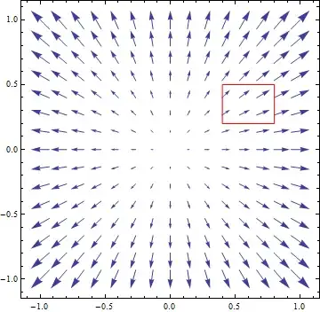
Here we see that the flow is aways from both axes, and actually is away from the origin. If we again look at a small rectangle somewhere in the first quadrant this time
we see that the outflow through the top wins the inflow at the bottom, and ALSO the outflow to the right wins the inflow from the left. Overall more stuff is flowing out than what's entering = positive divergence.
VectorPlot[{3 x, -3 y}, {x, -1, 1}, {y, -1, 1}]
was the Mathematica command that did the first plot.