Disclaimer. I find a few issues in the above question unclear. Therefore,
before doing any attempt to formulate a constructive answer
(@Piecewise parabolic) I'll ask some further questions.
Dirac-delta pair
Let's take an
extreme case of the "nonnegative smooth function"
$f : [0,1] \to {\mathbb R}^{+}$ , namely two
Dirac-delta's placed at $x_1$ and $x_2$ such that $0 \le x_1 < x_2 \le 1$:
$$
f(x) = A\, \delta(x-x_1) + B\, \delta(x-x_2)
$$
Physics intuition tells that the moment (of inertia/variance) is maximal which such
a configuration, because "mass is concentrated at the edges" :
$$
m_0 = A + B \quad ; \quad m_1 = A x_1 + B x_2 \quad ; \quad m_2 = A x_1^2 + B x_2^2
$$
Common mean $\mu$ and variance $\sigma^2$ are calculated from these:
$$
\mu = \frac{m_1}{m_0} = \frac{A x_1 + B x_2}{A+B} \\
\sigma^2 = \frac{m_2}{m_0} - \left(\frac{m_1}{m_0}\right)^2 = \frac{AB}{(A+B)^2}(x_2-x_1)^2
$$
It's no restriction on generality if we put $\,A=m_0 w\,$ and $\,B=m_0(1-w)\,$ in here. Then:
$$
\sigma^2(w) = w(1-w)(x_2-x_1)^2 \quad \Longrightarrow \quad \mbox{maximal for } \; w=1/2
$$
Giving for the square root of the variance, which is the
spread $\sigma$ :
$$
\sigma = \frac{1}{2}(x_2 - x_1) \quad \Longrightarrow \quad \mbox{maximal for} \; (x_1,x_2) = (0,1) \quad \Longrightarrow \quad \sigma_\mbox{max} = \frac{1}{2}
$$
And this is an extreme case. Any other and "smoother" function is expected to have a spread that is smaller.
With other words, the mean plus or minus the spread ($\mu\pm\sigma$) must be at the interval $[0,1]$.
However, it's quite easy,
with the conditions imposed by the OP's question, to go beyond all this.
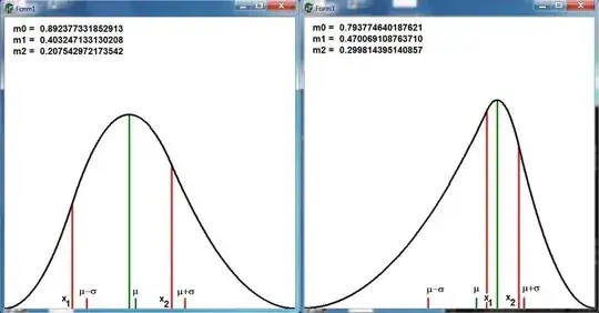
Here are two numerical examples:
$$
\left. \begin{array}{l}
m_0 = 0.988937212154269 \\
m_1 = 0.774045115569606 \\
m_2 = 0.749572664033622
\end{array} \right\} \quad \Longrightarrow \quad \left\{ \begin{array}{l}
\mu+\sigma = +1.16392865228137 \; \color{red}{> \, 1} \\ \mu-\sigma = +0.401479355540383 \end{array} \right.
$$ $$
\left. \begin{array}{l}
m_0 = 0.746407221304253 \\
m_1 = 0.080351584125310 \\
m_2 = 0.076326573966071
\end{array} \right\} \quad \Longrightarrow \quad \left\{ \begin{array}{l}
\mu+\sigma = +0.408765490356821 \\
\mu-\sigma = -0.193463221482986 \; \color{red}{< \, 0}
\end{array} \right.
$$
So the
question is: shouldn't the conditions on $\;m_0 , m_1 , m_2\;$ be
more restrictive in the first place?
Anyway,
with some restrictions as proposed, the solution of the OP's problem, with an
extremely unsmooth function instead of the desired smooth one, can be easily found:
$$
f(x) = \frac{m_0}{2}\left[\delta(x-x_1)+\delta(x-x_2)\right] \qquad \mbox{where} \quad
x_{1,2} = \mu\pm\sigma = \frac{m_1}{m_0} \pm \sqrt{\frac{m_2}{m_0} - \left(\frac{m_1}{m_0}\right)^2}
$$
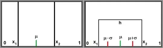
Rectangle
Before proceeding to the final part, let's consider a somewhat less extreme function
$f : [0,1] \to {\mathbb R}^{+}$ namely a
rectangle with height $h$ between
$x_1$ and $x_2$ :
$$
f(x) = \left\{ \begin{array}{lll}
0 & \mbox{for} & 0 \le x < x_1 \\
h & \mbox{for} & x_1 \le x \le x_2 \\
0 & \mbox{for} & x_2 < x \le 1 \end{array} \right.
$$
Not exactly what the OP wants, but somewhat closer (hopefully). The moments are:
$$
m_0 = h(x_2-x_1) \quad ; \quad m_1 = h(x_2^2-x_1^2)/2 \quad ; \quad m_2 = h(x_2^3-x_1^3)/3
$$
Common mean $\mu$ and variance $\sigma^2$ are calculated from these:
$$
\mu = \frac{m_1}{m_0} = \frac{x_1 + x_2}{2} \\
\sigma^2 = \frac{m_2}{m_0} - \left(\frac{m_1}{m_0}\right)^2 = \frac{(x_2-x_1)^2}{12}
$$
With the inverse problem, there are three unknown quantities $(x_1,x_2,h)$ and three equations:
$$
x_1^2 + x_1 x_2 + x_2^2 = 3 \frac{m_2}{m_0} \quad ; \quad
x_1 + x_2 = 2 \frac{m_1}{m_0} \quad ; \quad h(x_2-x_1) = m_0
$$
Giving as the solution ( with $\,x_2 > x_1$ ) :
$$
x_{1,2} = \frac{m_1}{m_0} \pm \sqrt{3} \times \sqrt{\frac{m_2}{m_0} - \left(\frac{m_1}{m_0}\right)^2}
\qquad \Longrightarrow \qquad h = \frac{m_0}{x_2-x_1}
$$
Note that, apart from a factor $\sqrt{3}$, this is similar to the solution for the Dirac-delta pair.
However, the factor $\sqrt{3}$ makes the conditions to be imposed upon the moments $\;(m_0,m_1,m_2)\;$
even more restrictive. It follows from $\,0 \le x_1 < x_2 \le 1\,$ that:
$$
0 < \mu - \sqrt{3}\,\sigma < \mu + \sqrt{3}\,\sigma < 1 \qquad \mbox{instead of} \qquad
0 < \mu - \sigma < \mu + \sigma < 1
$$
A general pattern seems to emerge:
with "neater" functions, there are more restrictive conditions
for the moments.
Piecewise parabolic
Hopefully our last function $f : [0,1] \to {\mathbb R}^{+}$
will fit the bill. Define as follows:
$$
f(x) = \left\{ \begin{array}{ll}
A x^2 & \mbox{for} \quad 0 \le x \le x_1 \\
a x^2 + b x + c & \mbox{for} \quad x_1 \le x \le x_2 \\
B(x-1)^2 & \mbox{for} \quad x_2 \le x \le 1
\end{array} \right.
$$
Here the coefficients $(A,B,a,b,c)$ must be such that the following conditions
are fulfilled:
$$
\begin{array}{l}
f(0) = 0 \quad \mbox{and} \quad f'(0) = 0 \quad \mbox{: automatically} \\
f(1) = 0 \quad \mbox{and} \quad f'(1) = 0 \quad \mbox{: automatically}
\end{array}
$$
$f(x)$ is continuous as well as differentiable in $x = x_1$ :
$$
f(x_1) = A x_1^2 = a x_1^2 + b x _1 + c \qquad ; \qquad
f'(x_1) = 2\,A x_1 = 2\,a x_1 + b
$$
$f(x)$ is continuous as well as differentiable in $x = x_2$ :
$$
f(x_2) = B(x_2-1)^2 = a x_2^2 + b x _2 + c \qquad ; \qquad
f'(x_2) = 2\,B(x_2-1) = 2\,a x_2 + b
$$
So far so good: is this
smooth enough?
At last,
the area under the whole curve $f(x)$ must be equal to $m_0$ :
$$
\int_{0}^{1} f(x) \, dx = m_0 \qquad \Longleftrightarrow \\
A x_1^3/3 + a (x_2^3 - x_1^3)/3 + b (x_2^2 - x_1^2)/2 + c (x_2 - x_1) + B (1-x_2)^3/3 = m_0
$$
There are five unknowns $(A,B,a,b,c)$ . And five equations have been found.
The solutions are:
$$
A = \frac{3 m_0}{x_1 x_2} \quad; \quad B = \frac{3 m_0}{1-x_1-x_2+x_1 x_2} \\
a = \frac{3 m_0 (-1+x_1-x_2)}{(-1+x_1) x_2 (-x_2+x_1)} \quad ; \quad
b = \frac{6 m_0}{(-1+x_1)(x_1-x_2)} \quad ; \quad c = \frac{-3 m_0 x_1}{(-1+x_1)(x_1-x_2)}
$$
Herewith all bits and pieces of the parabolas are found,
provided that the two coordinates $x_1$ and $x_2$ are known.
But, what we have instead is the inverse problem: two other moments $m_1$ and $m_2$ are known.
Which gives rise to two other equations. And these are non-linear, at least in principle:
$$
\int_{0}^{1} x f(x) \, dx = m_1 \qquad \Longleftrightarrow \\
\frac{A x_1^4}{4}+B\left(\frac{1}{12}-\frac{x_2^4}{4}+\frac{2 x_2^3}{3}-\frac{x_2^2}{2}\right)
+a\frac{x_2^4-x_1^4}{4}+b\frac{x_2^3-x_1^3}{3}+c\frac{x_2^2-x_1^2}{2} = m_1 \\
\int_{0}^{1} x^2 f(x) \, dx = m_2 \qquad \Longleftrightarrow \\
\frac{A x_1^5}{5}+B\left(\frac{1}{30}-\frac{x_2^5}{5}+\frac{x_2^4}{2}-\frac{x_2^3}{3}\right)
+a\frac{x_2^5-x_1^5}{5}+b\frac{x_2^4-x_1^4}{4}+c\frac{x_2^3-x_1^3}{3} = m_2
$$
However, it turns out that these equations, after substitution of $(A,B,a,b,c)$ ,
can be simplified
very much (and very much to my surprise too):
$$
x_1+x_2+1 = 4 \frac{m_1}{m0} \\
x_1^2+x_2 x_1+x_1+x_2^2+x_2+1 = 10\frac{m_2}{m_0}
$$
This is equivalent with
one quadratic equation for both $x_1$ and $x_2$ :
$$
x^2+\left[1-4\frac{m_1}{m_0}\right] x
+ \left[1-4\frac{m_1}{m_0}+16\left(\frac{m_1}{m_0}\right)^2-10\frac{m_2}{m_0}\right] = 0
$$
Which can be solved explicitly (again with $0 < x_1 < x_2 < 1$ ) :
$$
x_{1,2} = -\frac{1}{2}+2\frac{m_1}{m_0} \pm
\sqrt{-\frac{3}{4}+2\frac{m_1}{m_0}-12\left(\frac{m_1}{m_0}\right)^2+10\frac{m_2}{m_0}}
$$
Now substitute $(x_1,x_2)$ into $(A,B,a,b,c)$ and these into $f(x)$ and we're done.
Note, however, that the
restrictions upon the moments have become even more severe:
the expression under the square root must, of course, be positive and the condition
$0 < x_1 < x_2 < 1$ must stay fulfilled.
Conjecture
Definition. A non-negative smooth function $f : [0,1] \to {\mathbb R}^{+}$
is said to belong to $X$ if its moments $(m_1/m_0,m_2/m_0)$ are a member of the
set $X \subset {\mathbb R} \times {\mathbb R}$ . Four of these sets, namely $\{ E,D,R,P \}$ are defined as shown in the picture below.
 $$
E = \{ \color{gray}{gray} \} \cup \{ \color{blue}{blue} \}
\cup \{ \color{green}{green} \} \cup \{ \color{red}{red} \} \\
D = \{ \color{blue}{blue} \}
\cup \{ \color{green}{green} \} \cup \{ \color{red}{red} \} \\
R = \{ \color{green}{green} \} \cup \{ \color{red}{red} \} \\
P = \{ \color{red}{red} \}
$$
Less pictorial. Let $\frac{m_1}{m_0} = x$ , $\frac{m_2}{m_0} = y$ , $W = \sqrt{y-x^2}$ , $Q = \sqrt{-3/4 + 2 x - 12 x^2 + 10 y}$ . Then:
$$
E = \left\{ (x,y) \,|\, (x^2 < y) \wedge (y < x) \right\} \qquad D = \left\{ (x,y) \,|\, (0 < x-W) \wedge (x+W < 1) \right\} \cap E\\
R = \left\{ (x,y) \,|\, (0 < x- W\sqrt{3}) \wedge (x+ W\sqrt{3} < 1) \right\} \cap E \\ P = \left\{ (x,y) \,|\, (-\frac{3}{4}+2 x-12 x^2+10 y > 0) \wedge (0 < -\frac{1}{2} + 2 x - Q) \wedge (-\frac{1}{2} + 2 x + Q < 1)\right\}
$$
Conjecture.
$$
E = \{ \color{gray}{gray} \} \cup \{ \color{blue}{blue} \}
\cup \{ \color{green}{green} \} \cup \{ \color{red}{red} \} \\
D = \{ \color{blue}{blue} \}
\cup \{ \color{green}{green} \} \cup \{ \color{red}{red} \} \\
R = \{ \color{green}{green} \} \cup \{ \color{red}{red} \} \\
P = \{ \color{red}{red} \}
$$
Less pictorial. Let $\frac{m_1}{m_0} = x$ , $\frac{m_2}{m_0} = y$ , $W = \sqrt{y-x^2}$ , $Q = \sqrt{-3/4 + 2 x - 12 x^2 + 10 y}$ . Then:
$$
E = \left\{ (x,y) \,|\, (x^2 < y) \wedge (y < x) \right\} \qquad D = \left\{ (x,y) \,|\, (0 < x-W) \wedge (x+W < 1) \right\} \cap E\\
R = \left\{ (x,y) \,|\, (0 < x- W\sqrt{3}) \wedge (x+ W\sqrt{3} < 1) \right\} \cap E \\ P = \left\{ (x,y) \,|\, (-\frac{3}{4}+2 x-12 x^2+10 y > 0) \wedge (0 < -\frac{1}{2} + 2 x - Q) \wedge (-\frac{1}{2} + 2 x + Q < 1)\right\}
$$
Conjecture.
$P \subset R \subset D \subset E$ . None of the functions belong to $E\setminus D$ . All functions belong to $D$ . All (bump) functions with at most one maximum belong to $R$ . Only very specialized functions (I.e. piecewise parabolas) belong to $P$ .