Posted here by this author:
the question ,
a general answer, and a special answer.
You are reading the general answer now.
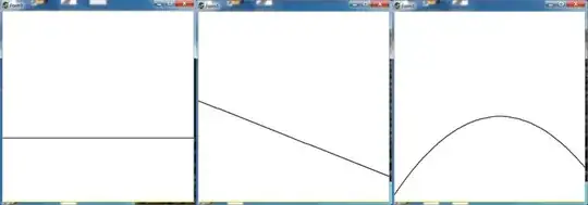
Suppose that we have a (real valued) function $f(x)$ defined WLOG at the interval $0 \le x \le 1$ and with moments $M_k$ , as described in the question. We have said nothing about $f(x)$ being positive, or smooth; the only obvious requirement being that it is integrable. A restriction $0 < M_k < 1$ on the moments, as proposed, does not simplify the problem much, admittedly.
Polynomial
Define a (real valued) polynomial $p(x) = a_0+a_1 x+ a_2 x^2 + \cdots + a_{n-1} x^{n-1} $ , at the same interval $0 \le x \le 1$ . The moments of the polynomial can be calculated easily:
$$
m_k = \int_0^1 p(x) x^k \, dx = \\ = a_0 \int_0^1 x^k dx + a_1 \int_0^1 x^{k+1} dx
+ a_2 \int_0^1 x^{k+2} dx + \cdots + a_{n-1} \int_0^1 x^{k+n-1} dx =\\ = \sum_{j=0}^{n-1} \frac{1}{j+k+1} a_j
$$
In matrix form:
$$
\left[\begin{array}{c} m_0 \\ m_1 \\ m_2 \\ \cdots \\ m_{n-1} \end{array}\right] =
\left[\begin{array}{ccccc} 1 & 1/2 & 1/3 & \cdots & 1/n \\
1/2 & 1/3 & 1/4 & \cdots & 1/(n+1) \\ 1/3 & 1/4 & 1/5 & \cdots & 1/(n+2) \\
\cdots & \cdots & \cdots & \cdots & \cdots \\ 1/n & 1/(n+1) & 1/(n+2) & \cdots & 1/(2n-1) \end{array}\right]
\left[\begin{array}{c} a_0 \\ a_1 \\ a_2 \\ \cdots \\ a_{n-1} \end{array}\right]
$$
Now suppose that the first $n$ moments of our function $f(x)$ are equal to the first $n$ moments of
the polynomial $p(x)$ , that is: $m_k = M_k$ for $k=0,1,2,\cdots,n-1$ .
Then we have $n$ equations with $n$ unknowns, which can be solved (theoretically) by matrix inversion:
$$
\left[\begin{array}{c} a_0 \\ a_1 \\ a_2 \\ \cdots \\ a_{n-1} \end{array}\right] =
\left[\begin{array}{ccccc} 1 & 1/2 & 1/3 & \cdots & 1/n \\
1/2 & 1/3 & 1/4 & \cdots & 1/(n+1) \\ 1/3 & 1/4 & 1/5 & \cdots & 1/(n+2) \\
\cdots & \cdots & \cdots & \cdots & \cdots \\ 1/n & 1/(n+1) & 1/(n+2) & \cdots & 1/(2n-1) \end{array}\right]^{-1}
\left[\begin{array}{c} M_0 \\ M_1 \\ M_2 \\ \cdots \\ M_{n-1} \end{array}\right]
$$
And we can actually find the (coefficients of the) whole polynomial from this limited subset of moments.
I said:
theoretically. Because the matrix to be inverted is recognized as the infamous
Hilbert
matrix. The Hilbert matrix is notorious for its bad conditioning, which means in practice that its inverse
can only be obtained with pain, namely at the cost of losing many significant digits.
Now forget about the moments for a moment :-)
With a Least Squares Method, on the other hand, the following integral is minimized:
$$
\int_0^1 \left[ f(x)-p(x) \right]^2 dx = \int_0^1 \left[ f(x)-\sum_{k=0}^{n-1} a_k x^k \right]^2 dx =
\mbox{minimum}(a_0,a_1,a_2,\cdots,a_{n-1})
$$
Take partial derivatives $\partial/\partial a_k \; ; \; k=0,1,2,\cdots,n-1$ to find the minimum:
$$
\int_0^1 x^k \left[ f(x) - \sum_{j=0}^{n-1} a_j x^j \right] dx = 0 \quad \Longleftrightarrow \quad
\sum_{j=0}^{n-1} \frac{1}{k+j+1} a_j = M_k
$$
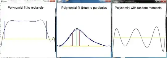
Which turns out to be exactly the same system of linear (and ill-conditioned) equations as above. Thus we conclude that finding a polynomial with the same first $n$ moments of a given function is equivalent with finding the least squares best fit polynomial of order $(n-1)$ to that function, WLOG at the interval $\left[0,1\right]$ . Now take the limit for $n\rightarrow\infty$ and we're done, it seems. So, any real valued function defined at a finite interval can be resolved (in a least squares sense) from its sequence of moments and there are no restrictions on these moments. It is noted that the functions found are, in general, no probability distributions and can be quite "wild".
At last, there is a residual (i.e. error estimate) to take into account:
$$
\int_0^1 \left[ f(x)-p(x) \right]^2 dx = \int_0^1 f(x)^2 dx - 2 \sum_{k=0}^{n-1} a_k \int_0^1 f(x) x^k dx
+ \sum_{k=0}^{n-1} a_k \sum_{j=0}^{n-1} a_j \int_0^1 x^k x^j dx = \\ = \int_0^1 f(x)^2 dx - \sum_{k=0}^{n-1} a_k M_k
$$
It is worrysome that, sometimes but too often, the residual turns out to be negative (numerically). How can that happen?
I think it means that our numerical calculations just aren't much reliable, due to poor condtioning of the Hilbert matrix.
Histogram
Define a (real valued) histogram $h(x)$ , at the same interval $0 \le x \le 1$ . Take equal intervals to begin with:
$$
h(x) = f_j \quad \mbox{for} \quad j/n < x < (j+1)/n \quad ; \quad j=0,1,2,\cdots,n-1
$$
The moments of the histogram can be calculated easily:
$$
m_k = \int_0^1 h(x) x^k \, dx = \sum_{j=0}^{n-1} f_j \int_{j/n}^{(j+1)/n} x^k \, dx =
\frac{1}{k+1}\sum_{j=0}^{n-1} \left[ \left(\frac{j+1}{n}\right)^{k+1}-\left(\frac{j}{n}\right)^{k+1}\right] f_j
$$
Now suppose that the first $n$ moments of our function $f(x)$ are equal to the first $n$ moments of
the histogram $h(x)$ , that is: $m_k = M_k$ for $k=0,1,2,\cdots,n-1$ .
Then we have $n$ linear equations with $n$ unknowns, which can be solved (theoretically).
So we can actually find the whole histogram from this limited subset of moments.
I said:
theoretically. Because the linear equations to be solved are ill conditioned again; maybe the
corresponding matrix is even worse than the Hilbert matrix.
With histogram functions, there is NO equivalent between the Moment problem and Least Squares:
$$
\int_0^1 \left[ f(x) - h(x) \right]^2 dx = \sum_{k=0}^{n-1} \int_{k/n}^{(k+1)/n} \left[ f(x) - f_k \right]^2 dx = \mbox{minimum}(f_0,f_1,f_2,\cdots,f_{n-1})
$$
Take partial derivatives $\partial/\partial f_k \; ; \; k=0,1,2,\cdots,n-1$ to find the minimum:
$$
\int_{k/n}^{(k+1)/n} \left[ f(x) - f_k \right] dx = 0 \quad \Longleftrightarrow \quad
\frac{\int_{k/n}^{(k+1)/n} f(x)\, dx}{(k+1)/n-k/n} = f_k
$$
Meaning that any $f_k$ is the mean of the function $f(x)$ over the interval $\left[k/n,(k+1)/n\right]$ .
At last, there is a residual (i.e. error estimate) to take into account:
$$
\int_0^1 \left[ f(x)-h(x) \right]^2 dx = \int_0^1 f(x)^2 dx - \sum_{k=0}^{n-1} \left[\frac{k+1}{n}-\frac{k}{n}\right] f_k^2
$$
Numerical calculations with Histogram Moments reveal that the results seem to be approximately what
one would expect with Least Squares (see: Histogram fit to parabolas). But it is not at all obvious
(to me at least) that the two methods converge to the same thing.
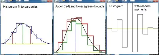
It is also possible to have
histograms as $\color{red}{upper}$ and $\color{green}{lower}$ bounds to a function.
Then the (raw) moments of the function are in between the (raw) moments of the histograms.
Given an infinite precision computer that does not suffer from ill conditioned equations, then
for $n\to\infty$ this fact would prove that an infinite sequence of moments determines the function.
It is shown in the picture, though, that solving the histogram equations gives $\color{red}{upper}$
and $\color{green}{lower}$ histograms that are seen to be different from the exact ones, thus confirming again the dreadful conditioning with even moderate size (< $10$) of the equations system. References: