Is there an explicit form for cubic Bézier curves?

Question

(See edits at the bottom)

I'm trying to use Bézier curves as an animation tool. Here's an image of what I'm talking about:

Basically, the value axis can represent anything that can be animated (position, scaling, color, basically any numerical value). The Bézier curve is used to control the speed at which the value is changing as well as it start and ending value and time. In this graphic, the animated value would slowly accelerate to a constant speed, then decelerate and stop.

The problem is, that Bézier curve is defined with parametric equations.

$f_x(t):=(1-t)^3p_{1x} + 3t(1-t)^2p_{2x} + 3t^2(1-t)p_{3x} + t^3p_{4x}$

$f_y(t):=(1-t)^3p_{1y} + 3t(1-t)^2p_{2y} + 3t^2(1-t)p_{3y} + t^3p_{4y}$

What I need is a representation of that same Bézier curve, but defined as value = g(time), that is, y = g(x).

I've tried solving for t in the x equation and substituting it in the y equation, but that 3rd degree is giving me some difficulty. I also tried integrating the derivative of the Bézier curve (dy/dx) with respect to t, but no luck.

Any ideas?

Note : "Undefined" situations are avoided by preventing the tangent control points from going outside the hull horizontally, preventing any overlap in the time axis.

EDIT : I have found two possible solutions. One uses Decasteljau's algorithm to approximate the $s$ parameter from the $t$ parameter, $s$ being the parameter of the parametric curve and $t$ being the time parameter. Here (at the bottom).

The other, from what I can understand of it, recreates a third degree polynomial equation matching the curve by solving a system of linear equation. Here. I understand the idea, but I'm not sure of the implementation. Any help?

Answer 1

You're really looking for a cubic equation in one dimension (time).

$$ y = u_0(1-x)^3 + 3u_1(1-x)^2x + 3u_2(1-x)x^2 + u_3x^3 $$

Is all you need.

Walking $t$ at even intervals (say in steps of 0.1) takes evenly spaced points along the parametric curve.

So, the answer to your question is really quite simple. The parametric bezier curve provides 2 variables as the output, with only 1 variable as the input. To control an animation in time like these, that's only a 1 dimensional situation. So consider $t$ as time, and drop one variable (say drop $x$). Your animation ease curve is controlled by the $y$ value:

Now as $t=0,0.1..1$, you have an animation parameter that starts slowly, moves at medium speed in the middle, and slows down at the end.

---

Examples

Setting $u_0=0$, $u_1=0.05$, $u_2=0.25$, $u_3=1$ gives an ease-in curve (slow start, fast end)

Setting $u_0=0$, $u_1=0.75$, $u_2=0.95$, $u_3=1$ gives an ease-out curve (fast start, slow end)

Answer 2

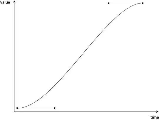
You don't want that! You want this!

'Eased' motion and 1D Beziers

You can solve a cubic, but it's tricky and probably not what you want

The fact that a cubic generally has three solutions is a big clue that 2D Beziers are powerful enough to draw totally inappropriate graphs for a single-valued function like yours.

(By a single-valued function I mean one that won't ever wrap back on itself in the x-direction.)

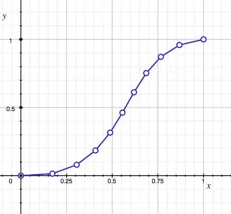
If you're looking for an attractive interpolation of discrete values, however, 2D Beziers are very convenient, especially as they're implemented in almost all drawing packages; so indeed 2D Beziers often are used to draw graphs of single-valued functions.

In such a case, it is best to make sure that each Bezier's two control handles share their horizontal coordinate, which would always lie halfway between the horizontal coordinates of the Bezier's end points. And that will cause the horizontal coordinate to vary linearly with t, and NOT as a cubic.

That effectively limits the possibilities of a 2D Bezier to those of a 1D Bezier. It's much more appropriate for a single-valued function, and of course makes it much easier to find y in terms of x.

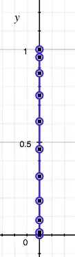
Consider a 1D equivalent

Not all Beziers are as much as 2D. In fact, easing (the technical name for the motion you are trying to achieve) is usually achieved with a 1D Bezier. There is even a specification in SVG for defining a custom easing on an animation, by specifying the end values and control values for a 1D Bezier.

Control values, in 1D as in 2D, are end values plus some difference value, which is related to the desired gradient of the dependent variable, with respect to the independent variable. In particular, it happens to be exactly half the desired gradient. In your case, you want a gradient of zero at both ends of the eased motion, so your control values should be the same as your end values. (This corresponds to the fact that your control handles are horizontal, giving a zero gradient of y with respect to the independent variable.)

Option 1: Construct a polynomial and step through it with constant time increments

If you have a pair of values and their gradients with respect to the independent variable, you can interpolate them with a Cartesian cubic, in the form

y = a.t^3 + b.t^2 + c.t + d

If you decide on values for more derivatives, the same method can lead you to higher orders of polynomial. So to specify end accelerations, you need the versatility of a 5th order polynomial, and to specify jerk and jounce, you need the 7th and 9th orders respectively. This adds expressiveness to the curve without requiring you to find the roots of anything!

I'll explore the method here for just the cubic version.

This is effectively a one dimensional case of what you would do to construct a 2D Bezier. Again, you are fixing a position and a gradient at each end of the curve.

For some extra background: The control handles you're used to, on a 2D Bezier, automatically determine the gradients of x and y with respect to the independent variable t. The gradients are twice the size of the horizontal and vertical components, respectively. (Scaling them together, away from this value, gives other valid curves of the same order, maintaining the tangent direction, but they would compromise the recursive interpolation properties of a Bezier and its hull.)

In a 1D case, you need to decide the gradient of y with respect to x, by whatever means is appropriate for your application. There are many algorithms you could choose for that. It is just like choosing the positions of control handles. In your case, you want a gradient of zero at both ends of the easing.

Once you've chosen your end values, you have some (fairly simple) simultaneous equations to determine the values of a, b and c.

To make things easier, let's suppose that t runs from 0 to 1. I would recommend implementing it this way; actual time values for a particular animation can be mapped to and from this time-scale as needed. So if the actual animation starts at start and lasts for duration, just use

T = start + duration.t and t = (T - start)/duration

to convert.

That way, at one end of the line, the equations for y and its gradient,

y = a.t^3 + b.t^2 + c.t + d
dy/dt = 3a.t^2 + b.t + c

simply collapse all the way down to

y = d
dy/dt = c

So from the value of the function and the decided-on gradient at t = 0, you already have two terms of the polynomial. At the t = 1 end of the motion, we find

1. y = a + b + c + d
2. dy/dt = 3a + 2b + c

and finding a and b by elimination is now easy.

Equation 2. - 2 x Equation 1. to eliminate b and calculate a
3 x Equation 1. - Equation 2. to eliminate a and calculate b

Option 2: Use in-built Bezier functionality, and just specify end/control values

This would probably be done most easily by more thoroughly investigating the easing functions available to you in the language you're using.

My personal fallback, if there is no such functionality, would be the above method of finding a suitable polynomial to step through.

But you already appear to be almost there, with your solution, so I can't resist adding what is needed, to complete it.

So you can clearly can draw a Bezier somehow. And you appear to have decided to get one coordinate of that Bezier -- again, somehow -- so then you can use it as your easing value. Okay.

Modify your particular Bezier to be linear in the horizontal axis

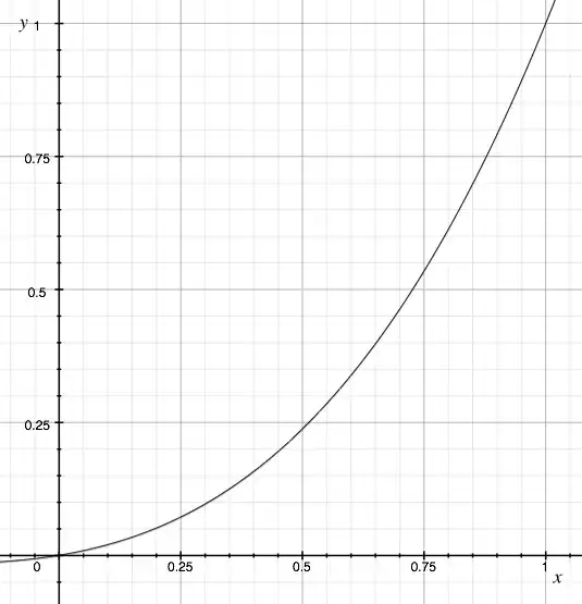
Certain special cases of Bezier are worth noting here.

1. When the control points have identical x values, x will only be quadratic in t. Likewise, if they have identical y values, y will only be quadratic in t. When both components are identical (so there is only one, shared control point), the Bezier is entirely quadratic.
2. When the shared x value is equidistant between the end points, x will only be linear in t. Likewise, if a shared y value lies halfway, y will only be linear in t. For a shared control point halfway between the end points, the Bezier is entirely linear. (The curve is straight and is traced at constant speed.)

So by setting the x coordinates of the control handles to be halfway between the x coordinates of the end points, you will construct the special case that has the parametric form

x = a.t^3 + b.t^2 + c.t + d, with a = 0, b = 0 making it LINEAR
y = e.t^3 + f.t^2 + g.t + e

Once again, you now have a linear relationship between x and t, so you can easily express y in terms of x by making a substitution in the explicit expression for y.

Because I Don't Like To Leave Anything Unanswered...

Do you still have need of a cubic solver? And can you say more about your difficulties?

A word of warning about naive equations

You definitely do want to solve the linear equation AS a linear equation. Don't be thinking that something more general must also work on lower orders of equation. Even if you write a cubic solver, it will actually break in this case.

Trying to solve a lower order equation with techniques for higher orders will tend to lead you into a division by zero. In a simpler case, consider solving the linear equation,

B.t + C = 0

with the general formula for quadratics,

t = (-B +- sqrt(B^2 - 4A.C)) / 2A, with A = 0

This gives the answers finite/zero and zero/zero, which aren't particularly useful even if you can interpret them as correct. Each is easy to understand if you watch what happens to the solutions as the value of A vanishes.

Another word of warning about cubic and quartic solvers

A lot is already available on how to do this, either symbolically or numerically. I can't add much here, to what's already available, especially with the scant clues I have about what level you're at. (You haven't said much about your progress so far.)

But the standard warnings bear repeating:

1. Symbolic solvers are often slower at achieving the same accuracy.
2. When you vary the terms of the polynomial smoothly, the true roots should vary smoothly, but the calculated roots often won't, being sensitive to rounding errors in your calculation. (That's mainly true of the symbolic solvers.) This is what is meant by the 'numeric stability' of your roots. You want smooth motion so this is an issue.
3. Are you sure you want to spend performance on root finding, in the inside loop of an animation, given the huge number of explicit functions you could use for easing?

Answer 3

The basic required function is $y = 3x^2 - 2x^3$.

This is a smooth "ramp" that rises from $y=0$ at $x= 0$ to $y = 1$ at $x=1$.

You can then shift it and scale it to suite your needs.

This is a real-valued Bezier curve that has "control points" $\left(0, 0\right), \left(\frac{1}{3}, 0\right), \left(\frac{2}{3}, 1\right), \left(1, 1\right)$.

Answer 4

Notice that if you happen to have $p_{1y}=0$, $p_{2y}=1/3$, $p_{3y}=2/3$ and $p_{4y}=1$, so that $f_y(t)=t$, then the graph you are after is actually of the inverse function of $f_x(t)$, which is going to be a mess and inevitable as complicated as the usual formula for the roots of a cubic polynomial.

That shows that the general formula necessarily has to be complicated. I doubt there is anything useful to be done...

Answer 5

I Probably Shouldn't Do This

My previous answer made clear that I think your question was the wrong question. But on principle, I can't leave it at that; I will answer the question anyway...

If you're really determined to draw shapes with your familiar Bezier tools, and to use one coordinate of a resulting curve as an easing value, I recommend that you use one of the following methods:

Numerically solve the polynomial P(t) - x = 0 to find t, using an end point as a 'first guess'.

You already know a solution at each end of the curve. Either of those is a good first guess for the next or previous value, which is a good first guess for the next value you want, and so on. That means you can use a numerical solver very quickly and accurately, and usually only finding one root.

You hinted at a similar solution, but you didn't seem very happy with it, calling it 'a bit hacky'. Here I mean to get you thinking more clearly about it, because it needn't bit at all hacky, and can be both quite fast as well as the most accurate.

Wikipedia's page on root finding algorithms has many possibilities to suggest, and you needn't even bother assessing their relative merits much; go with whatever you find easy to implement. Having a first guess to hand means lots of methods work very, very well in terms of both speed and accuracy.

For values of x that correspond to multiple different values of t, the value of t that is closest to your previous value will be found, and that seems desirable. The only question then is how to behave when the value you've been tracking vanishes.

Consider drawing an upright S shape on the graph in your example. Scanning from left to right, we start with only one solution, but then two more appear in a manner reminiscent of a particle-antiparticle creation. What is the definition of the behaviour you desire, in such cases?

At this stage most root finding algorithms will continue to return the t value corresponding to the bottom-most root. But when the original root and the middle root collide, they annihilate, again in a way reminiscent of particles and antiparticles.

What happens there depends a bit more on your choice of root solver. In most cases there will be two consequences. Usually, the root will simply jump to the top of the S, and take slightly more calculation time on that step. (Tracing back to the left will then stay on the top of the S.) For some choices of root finder, you could run into a bigger problem here, like the root finder no longer converging on any root, because the initial guess was too far away.

If you actually want to know about all the possible roots, that takes a bit more work. By removing a factor of (t - root) from the polynomial P(t) - x you will get a lower order expression, making it successively easier to find subsequent roots. But the division is difficult, and the accuracy of each subsequent root tends to be much worse than the last one. I would use these subsequent calculations of roots as first guesses for a further numerical iteration.

If you think multiple roots won't affect you for the curves you're likely to draw, because you're drawing single-valued functions, beware. Just because there is a single valid solution in the curve segment you've drawn, doesn't mean the root finder won't discover other solutions from outside it. The fact that the equation potentially has three roots makes your calculation harder even if only one is real, or only one is in the valid t domain.

And Here's Another Way

First, notice that the quadratic Bezier is a much easier case. You can get both solutions of t for every value of x from the quadratic formula, and making a consistent choice of root is easy.

So how closely can you approximate one cubic Bezier with many quadratic Beziers?

If using this method, remember that while any one subdivision can now give a maximum of two roots, the entire curve could have a total of three.

But HONESTLY You're Better Off With These!

Calculating polynomial expressions is easy, 'forward' mathematics; rooting finding is difficult, 'backwards' mathematics. Go forwards; make it easy for you AND for the computer; don't calculate roots for such a basic component of animation as easing.

As suggested by bubba:

Cubic easing from 0 to 1, over t = 0 to t = 1
ease = 3t^2 − 2t^3

Cubic easing from -1 to 1, over t = -1 to t = 1
ease = (3t - t^3)/2

These trig solutions also look nice. Trig is quicker if you calculate each sin(t) from the cos and sin of the previous t with some linear algebra; I advise doing so in any inside loop of an animation

Harmonic easing from 0 to 1, over t = 0 to t = 1:
ease = (1 + sin(pi.(2t - 1))) / 2

Harmonic easing from -1 to 1, over t = -1 to t = 1:
ease = sin(pi.t)

You can still have an intuitive, graphical interface for designing lots of these functions.

If control points are horizontally fixed, your graph would actually provide a nice way to design a 1D Bezier of any order at all, with the independent variable represented on the horizontal axis.

With that one 'restriction' it would be a very intuitive interface for setting positions and velocities. It would be nice to extend that into an interface for providing velocities and accelerations, and then accelerations and jerks, and then jerks and jounces. Each new graph can provide positions from the previous graph, and just needs the gradients to be added.

And nobody could criticise that for a lack of 'expressiveness'!

Answer 6

Assuming the intended meaning of $p1x$, etc. was as Ross believed, you should be able to solve for t explicitly in either equation using the formula at http://en.wikipedia.org/wiki/Cubic_equation#General_formula_of_roots. Of course, this is a bulky solution and you would need to identify which solution is real (though there should be only 1 assuming that the curve can be represented as $y = g(x)$).

Answer 7

Any implicit Cartesian equation you'll attempt to derive from the Bézier curve is necessarily complicated because the explicit solution for the cubic equation is complicated, as explained by other answers; if you desperately need a $y=f(x)$ for manipulations, you're probably better off constructing a (piecewise) Hermite interpolant, which assumes you have an appropriate number of derivatives available in addition to function values.

For the cubic case, one only needs two triples $(x_i,y_i,y_i^\prime)$ and $(x_{i+1},y_{i+1},y_{i+1}^\prime)$ available; then, there is a unique cubic $p_3(x)$ that satisfies the conditions $p_3(x_i)=y_i$ and $p_3^\prime(x_i)=y_i^\prime$ (and similarly for the other triple). If, say, you have $y_i$ as position values and $y_i^\prime$ as velocity values, you're all set. If you additionally have second derivative values, you can construct a quintic, but since that sort is rarely needed/wanted, a cubic usually suffices.

Note that cubic splines are but a special case of cubic Hermite interpolation; the additional thing is that continuity conditions (the agreement of first and second derivative values at certain points) are implemented.

Answer 8

I tried the two solutions I've linked to the original question (Solution 1 and Solution 2). Here are my results.

Solution 1

The idea is to recreate the curve with a third degree polynomial, by matching the value at P1 and P4 and their respective slope. This polynomial can be solve using a system of linear equations. The only problem is that it's possible to create an infinite slope at P1 or P4 with the Bezier curve, which is impossible to recreate with the polynomial. I've also tried using a 5th degree polynomial (matching value, first derivative and second derivative) without success, because it has the same problem.

Solution 2

This solution is pretty simple, but a bit hacky. The idea is to use the De Casteljau algorithm to search for a t (parameter of the Bézier curve) that matches a given x variable (x-axis). The algorithm is simple :

1. Split the curve in half
2. Is the x of the split point is approximatively equal to the searched x? If yes, return t
3. Else, if the searched x is greater that the x of the split point, repeat the algorithm with the segment on the right, else on the left.

Once you have the t, you can obtain the y value using the Bézier function $f_y(t)$ in my original post.

So, yeah, working, but a bit hacky.