5

Parabolic interpolation is an easy way to estimate the maximum of a function known by three values at equally spaced points, the central value being the largest.

Is there an easy way to generalize this to 2 dimensions or more, knowing the function values on a regular square lattice ($3^d$ points) ?

(A multiparabolic interpolation is possible, but leads to high order equations; a quadric equation doesn't have enough degrees of freedom.)


Update:

One can reason on interpolating basis functions, such that they are zero on all points but one. In 1D, this can be achieved with parabolas. In 2D higher order functions are unavoidable, as there are 9 constraints. Quadrics can't achieve this. Cubics do not seem to be the right choice, as they have 10 coefficients.

  • Just a speculation: what if you try to do a parabolic least square fitting instead of the exact interpolation? – A.Γ. Nov 08 '17 at 11:21
  • @A.Γ.: that's an option, but I prefer an interpolation. –  Nov 08 '17 at 11:23
  • There is a somewhat different formula in my answer, not equivalent with yours : $\hat x=\frac{(y_+-y_-)/2}{2y_0-y_+-y_-}$ . Which one is the right one? – Han de Bruijn Nov 11 '17 at 19:43
  • @HandeBruijn: I don't see any difference !? –  Nov 11 '17 at 19:45
  • And shouldn't the last formula be : $\hat y=\frac{y_-}2\hat x(\hat x-1)-y_0(\hat x-1)(\hat x+1)+\frac{y_+}2(\hat x+1)\hat x.$ ? – Han de Bruijn Nov 11 '17 at 19:49
  • Isn't $,y_+-y_-,$ different from $,(y_+-y_-)/2$ ? – Han de Bruijn Nov 11 '17 at 19:52
  • @HandeBruijn: I have removed the formulas, which are unimportant. –  Nov 12 '17 at 09:18
  • No, your formulas weren't unimportant. And, obviously, I do not support your update, where it is stated that "Quadrics can't achieve this". Which is in blatant contradiction with my answer. – Han de Bruijn Nov 12 '17 at 11:17

3 Answers3

2

An easy way is proposed by Han de Bruijn, which basically tries to find the minimum location per dimension (correct me if I am wrong). However, in that case you are not using all information you have, so it is definitely not optimal in that sense. On the other hand, I don't think there is an easy way if you want to use all data points. Below, I present the easiest way I could come up with to compute the minimum (apologies, but I find it way easier to think of a minimum instead of a maximum).

Let $y \in \mathcal{R}$ be the output of the function for which you want to find a parabolic fit and let $\bar{x} \in \mathcal{R}^d$ be the location of the optimum, i.e. where the gradient is zero. The dimension is denoted by $d$. In that case, we can approximate $y$ using our parabolic function: $$ y = (x - \bar{x})^T A (x - \bar{x}) + c $$ Here, $x\in\mathcal{R}^d$ denotes the input vector, $A\in\mathcal{R}^{d\times d}$ is a symmetric positive definite matrix (in case of maximization, A has to be negative definite) and $c$ is the value of $y$ at the optimum (i.e., if $x=\bar{x}$). We have $(d+1)(d+2)/2$ unknowns.

You can see that this is not straightforward to solve, as we end up with a cubic term $\bar{x}^TA\bar{x}$. For example, with least squares you can still solve this, given your datapoints $(x_1, y_1), ..., (x_N, y_N)$, with $N=3^d$. To this end, let this be the cost function you want to minimize: $$ J(\bar{x}, A, c)=\sum_{i=1}^N \left( (x_i-\bar{x})^TA(x_i-\bar{x})+c-y_i\right)^2 $$ Through minimization of $J(\bar{x}, A, c)$, you can find the location of the optimum $\bar{x}$ and the minimum value of $y$, i.e. $c$.

I tried to write a simple function in python, which takes as input the data and the dimension $d$. I tried it for $d=4$ and it comes instantly with a solution, so I think it should also handle $d=6$ well enough. I hope it helps you.

import numpy as np
from scipy import optimize


class ParabolicInterpolation:
    def __init__(self, ndim):
        """Initialize parabolic interpolation in n dimensions"""
        self.n = ndim
        self.datax = np.array([])
        self.datay = np.array([])
        self.r, self.c = np.triu_indices(self.n)  # Will be used to construct the A-matrix
        self.ahat = np.zeros((self.n, self.n))

    def get_x_a_c(self, x):
        """Return the offset x, the A matrix and the offset c"""
        xhat = x[:self.n]
        self.ahat[self.r, self.c] = x[self.n:-1]
        self.ahat[self.c, self.r] = x[self.n:-1]
        chat = x[-1]
        return xhat, self.ahat, chat

    def f(self, x):
        """Return the error between model and data"""
        xhat, ahat, chat = self.get_x_a_c(x)
        xoff = self.datax - xhat
        yhat = np.einsum('in,in->i', np.einsum('in,nj->ij', xoff, ahat), xoff) + chat  # Estimated output
        return yhat - self.datay

    def fit(self, datax, datay):
        """Compute the unknowns using Least Squares"""
        self.datax = datax
        self.datay = datay
        init = np.zeros(((self.n+1) * (self.n+2)) // 2)
        i = -1  # Make sure we start with identity matrix
        for j in range(self.n):
            i += self.n + 1 - j
            init[i] = 1
        xopt = optimize.leastsq(self.f, init)[0]
        xhat, ahat, chat = self.get_x_a_c(xopt)
        print("Minimum at: [", end="")
        for i in range(self.n):
            print("{:.2e}{:s}".format(xhat[i], ', ' if i+1 < self.n else ''), end="")
        print("]")
        print("Minimum value: {:.3e}".format(chat))
        return xopt


# Small demo
A = np.array([[1, 0.5, 0.25, 0.1], [0.5, 2, 0.25, -0.2], [0.25, 0.25, 1.5, -0.1], [0.1, -0.2, -0.1, 1]])
c = 0.5  # This is the minimum value we want to find
xstar = np.array([0.5, 0.25, -0.2, 0.6])  # This is the location of the minimum value

# Create some fake data
n = len(xstar)
X = np.zeros((3 ** n, n))  # Create the lattice square points
X[0, :] = -1
for ii in range(1, 3 ** n):
    X[ii] = X[ii-1]
    X[ii, 0] += 1
    jj = 0
    while X[ii, jj] == 2:
        X[ii, jj] = -1
        jj += 1
        X[ii, jj] += 1
y = np.zeros(X.shape[0])
for ii in range(X.shape[0]):
    y[ii] = np.dot(np.dot(X[ii]-xstar, A), X[ii]-xstar) + c
y += np.random.randn(X.shape[0])*0.05  # Add some noise, otherwise it is too simple ;)

# Perform the parabolic interpolation
pi = ParabolicInterpolation(n)
pi.fit(X, y)
EdG
  • 1,596
0

For an interpolation knowing the function values on a regular square lattice I don't know. But if you know the values on the vertices + mid-points on edges of a tetrahedron (in dimension $d$) then it is fairly easy (at least on a computer): In a suitable coordinate system you want to interpolate with: $$ p(x) = \sum_{1\leq i\leq j\leq d} a_{ij} x_i x_j + \sum_{1\leq i \leq d} b_i x_i + c $$ knowing the values $y_u$ on the set of points: ${\cal U} = \{ u= (u_1,...,u_d)\}$ where $u_i\geq 0$ and $\sum_i u_i \leq 2$. You have $(d+1)(d+2)/2$ points and the same number of constants. The kernel of the map $$p \mapsto \{p(u): u\in {\cal U} \}$$ is the zero-polynomial so it is a bijection. Thus given the values you may invert to obtain the interpolated quadratic polynomial. So for example in 2 dimensions you have the polynomial (6 coeffs): $$ p(x_1,x_2) = a_{11}x_1^2+a_{12}x_1x_2+a_{22}x_2^2+b_1x_1+b_2x_2 + c$$ and the 6 interpolation points: $$ {\cal U} = \{(2,0), (1,1), (0,2), (1,0), (0,1), (0,0) \} $$ Given the values on the set ${\cal U}$ you solve (easily on a computer) to get the polynomial. You may, of course, scale ${\cal U}$ to fit your purpose. Whether there is a max/min then depends upon the sign of the quadratic form which is by no means obvious to guess knowing the point values.

Edit: Given your comments, I guess you already used the interpolation on the product lattice $\Lambda$ with $3^d$ points by: $$ P(x) = \sum_{i_1=0}^2 \cdots \sum_{i_d=0}^2 a_{i_1,...,i_d} x_1^{i_1}\cdots x_d^{i_d}$$ which should give a bijection between the $3^d$ coefficients and values on $\Lambda$. However, computation of max/min is rather costly, in particular when the degree is quite large. In comparison, the tetrahedron approach yields a simple quadratic form for which max/min is much easier to obtain (a bit more work is needed if you want to test for max/min on the boundary of the polyhedron).

So adjusting your objective and work with triangularizations of your domain might be an idea? (or use Least Square method for the product lattice to approximate by the above quadratic form).

H. H. Rugh
  • 35,236
  • Thanks, but I am looking for a solution on $3^d$ points of a square lattice. This is not negotiable ;-) –  Nov 09 '17 at 21:47
  • ok, that is doable but not very nice. I believe that you can equally well interpolate for this, but with a degree $2^d$ polynomial. Computing max/min is probably beyond practical reach (for $d$ large). I can add details if you are interested. – H. H. Rugh Nov 09 '17 at 22:41
  • I have already used multiparabolic interpolation ($2^d$) and optimization by sequential 1D maximization. I am looking for something faster/simpler, if that exists. –  Nov 10 '17 at 08:00
  • Note that my $d$ is at most $6$, but is is already big ($729$ points). –  Nov 10 '17 at 09:21
0

Disclaimer. This answer is more or less a copy from material in

Quadrilateral Interpolation

enter image description here
Theory is specified for a rectangular square lattice, therefore isoparametric transformations are out of order here.
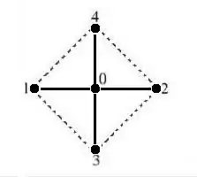
The above shape is known in Finite Difference circles as a five point star. Let its coordinates be given by: $$ (0) = (0,0) \quad ; \quad \begin{cases} (1) = (-1,0) \quad ; \quad (2) = (+1,0) \\ (3) = (0,-1) \quad ; \quad (4) = (0,+1)\end{cases} $$ Let function behaviour "inside" the five point star be approximated by a quadratic interpolation between the function values at the vertices or nodal points, let $T$ be such a function and use its Taylor expansion around the origin $(0)$: $$ T(x,y) = T(0) + \frac{\partial T}{\partial x}(0).x + \frac{\partial T}{\partial y}(0).y + \frac{1}{2} \frac{\partial^2 T}{\partial x^2}(0).x^2 + \frac{1}{2} \frac{\partial^2 T}{\partial y^2}(0).y^2 $$ Specify $T$ for the vertices with the basic polynomials of the five point star: $$ T_0 = T(0)\\ T_1 = T(0) - \frac{\partial T}{\partial x}(0) + \frac{1}{2} \frac{\partial^2 T}{\partial x^2}(0)\\ T_2 = T(0) + \frac{\partial T}{\partial x}(0) + \frac{1}{2} \frac{\partial^2 T}{\partial x^2}(0)\\ T_3 = T(0) - \frac{\partial T}{\partial y}(0) + \frac{1}{2} \frac{\partial^2 T}{\partial y^2}(0)\\ T_4 = T(0) + \frac{\partial T}{\partial y}(0) + \frac{1}{2} \frac{\partial^2 T}{\partial y^2}(0)\\ \quad \mbox{ F.E. } \leftarrow \mbox{ F.D. } $$ Solving these equations is not much of a problem and well-known Finite Difference schemes are recognized: $$ T(0) = T_0 \\ \frac{\partial T}{\partial x}(0) = \frac{T_2-T_1}{2}\\ \frac{\partial T}{\partial y}(0) = \frac{T_4-T_3}{2} \\ \frac{\partial^2 T}{\partial x^2}(0) = T_1-2T_0+T_2 \\ \frac{\partial^2 T}{\partial y^2}(0) = T_3-2T_0+T_4 \\ \quad \mbox{ F.D. } \leftarrow \mbox{ F.E. } $$ Finite Element shape functions may be constructed as follows: $$ T = N_0.T_0 + N_1.T_1 + N_2.T_2 + N_3.T_3 + N_4.T_4 = \\ T_0 + \frac{T_2-T_1}{2}x + \frac{T_4-T_3}{2}y + \frac{T_1-2T_0+T_2}{2}x^2 + \frac{T_3-2T_0+T_4}{2}y^2 =\\ (1-x^2-y^2)T_0 + \frac{1}{2}(-x+x^2)T_1 + \frac{1}{2}(+x+x^2)T_2 +\frac{1}{2}(-y+y^2)T_3 + \frac{1}{2}(+y+y^2)T_4 \\ \Longrightarrow \quad \begin{cases} N_0 = 1-x^2-y^2 \\ N_1 = (-x+x^2)/2\\ N_2 = (+x+x^2)/2\\ N_3 = (-y+y^2)/2\\ N_4 = (+y+y^2)/2 \end{cases} $$ So far so good concerning the generalities. Now specify for the problem at hand: $$ \frac{\partial T}{\partial x} = \frac{\partial T}{\partial x}(0)+\frac{\partial^2 T}{\partial x^2}(0).x = \frac{T_2-T_1}{2} + (T_1-2T_0+T_2).x = 0 \\ \Longrightarrow \quad x = - \frac{(T_2-T_1)/2}{T_1-2T_0+T_2} \\ \frac{\partial T}{\partial y} = \frac{\partial T}{\partial y}(0)+\frac{\partial^2 T}{\partial y^2}(0).y = \frac{T_4-T_3}{2} + (T_3-2T_0+T_4).y = 0 \\ \Longrightarrow \quad y = - \frac{(T_4-T_3)/2}{T_3-2T_0+T_4} $$ Substitute these $(x,y)$ values into either the F.D. or the F.E. formulation for $T(x,y)$ and you're done. The above can easily be generalized for multiple dimensions. As has been done in:

Linear isoparametrics with dual finite elements

For example a generalization to three dimensions, being the well-known seven point star: $$ (0) = (0,0,0) \quad ; \quad \begin{cases} (1) = (-1,0,0) \quad ; \quad (2) = (+1,0,0) \\ (3) = (0,-1,0) \quad ; \quad (4) = (0,+1,0) \\ (5) = (0,0,-1) \quad ; \quad (6) = (0,0,+1)\end{cases} $$ With accompanying interpolation: $$ T(x,y,z) = T_0 + \frac{T_2-T_1}{2}x + \frac{T_4-T_3}{2}y + \frac{T_6-T_5}{2}z\\ + \frac{T_1-2T_0+T_2}{2}x^2 + \frac{T_3-2T_0+T_4}{2}y^2 + \frac{T_5-2T_0+T_6}{2}z^2 $$ The place $\,(x,y,z)\,$ where the function $\,T(x,y,z)\,$ has its maximum is found by: $$ \frac{\partial T}{\partial x} = 0 \quad \Longrightarrow \quad x = - \frac{(T_2-T_1)/2}{T_1-2T_0+T_2} \\ \frac{\partial T}{\partial y} = 0 \quad \Longrightarrow \quad y = - \frac{(T_4-T_3)/2}{T_3-2T_0+T_4} \\ \frac{\partial T}{\partial z} = 0 \quad \Longrightarrow \quad z = - \frac{(T_6-T_5)/2}{T_5-2T_0+T_6} $$ At last substitute these $(x,y,z)$ values into the interpolation formula for $T(x,y,z)$ . Analogous procedure for $d$ dimensional space requires a stencil with $2d+1$ nodes, e.g. $13$ nodes for $d=6$.

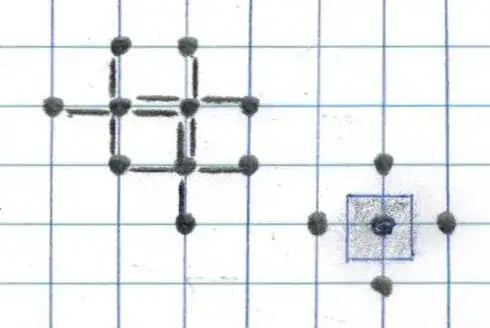
UPDATE. A picture says more than a thousand words:

enter image description here

It is seen that the five node stars in the grid have double chemical bonds, so to speak. This is the way all data points are actually available. However, there is some ambiguity involved in assigning the function values - already present in 1D. Which can be resolved by assigning a certain domain - shaded region around the central node $(0)$ - to each of the five node stars.

Han de Bruijn
  • 17,070
  • You are not using all datapoints which are available. I think it would be good to mention this. Furthermore, correct me if I am wrong, but basically you are fitting a 1D parabola for each direction independently. It is very simple (which is good, because that was the question), but I think you wrote it down in a rather complicated manner. Could you write it in a simpler (shorter) way? – EdG Nov 14 '17 at 14:07
  • @EdG: Sorry to inform you that I am using all data points. And I am fitting a 2D parabola for all directions. The shorter/simpler way of writing it down is found in the section below Linear isoparametrics with dual finite elements. I did it the way it has been done above that link because I want to spread a general message about geometrical shapes and interpolations. But anyway, I shall update the answer to clarify your first point. Be patient. – Han de Bruijn Nov 14 '17 at 17:38
  • @EdG: You're welcome to take notice of my update. – Han de Bruijn Nov 14 '17 at 20:05
  • Thanks for the update. You say you are using all data points. Aren't you referring to all datapoints that lie on a certain axis? For example, the datapoint $(1, 1, 1)$ is not used. Although it is not entirely clear for me, but I think in this problem, as there are $3^d$ datapoints, you are not using all datapoints which are available. Also, a 2D parabola, I don't see it, because you ignore terms $xy$, $xz$ and $yz$. Your partial derivatives gives the same formula's for 1D parabolic interpolation, so I don't see the why it is 2D. – EdG Nov 14 '17 at 23:21