Problem Statement
Modestly generalize the problem to consider underdetermined matrices of rank one.
Given
We are given the matrix $\mathbf{A}\in\mathbb{R}^{2\times 3}$ and the data vector $b\in\mathbb{R}^{2\times 1}_{1}$
$$
\mathbf{A} =
%
\left[
\begin{array}{rrr}
2 & -2 & 4 \\
-1 & 1 & -2 \\
\end{array}
\right], \quad
%
b =
\left[
\begin{array}{c}
3 \\
1
\end{array}
\right]
%
$$
and the goal is to find the set least squares minimizers for
$$ \mathbf{A} x = b.$$
The matrix $\mathbf{A}$ has $m=2$ rows, $n=3$ columns, and rank $\rho=1$. (There a few ways to resolve the rank. For example, notice that the two rows are linearly dependent.)
Least squares solution
The set of least squares minimizers is defined as
$$ x_{LS} = \left\{ x \in \mathbb{R}^{3} \colon
\lVert \mathbf{A} x_{LS} - b\rVert_{2}^{2} \text{ is minimized} \right\}.\tag{1}$$
Fundamental Theorem of Linear Algebra
The Fundamental Theorem of Linear Algebra provides fundamental insight. A matrix $\mathbf{A} \in \mathbb{C}^{m\times n}_{\rho}$ induces for fundamental subspaces:
$$
\begin{align}
%
\mathbf{C}^{n} =
\color{blue}{\mathcal{R} \left( \mathbf{A}^{*} \right)} \oplus
\color{red}{\mathcal{N} \left( \mathbf{A} \right)} \\
%
\mathbf{C}^{m} =
\color{blue}{\mathcal{R} \left( \mathbf{A} \right)} \oplus
\color{red} {\mathcal{N} \left( \mathbf{A}^{*} \right)}
%
\end{align}
$$
(Blue denotes vectors in a $\color{blue}{range}$ space, red denotes vectors in a $\color{red}{null}$ space.)
Focus on the structure of the domain space. Because $\rho<n$, the null space is nontrivial:
$$ \color{red}{\mathcal{N} \left( \mathbf{A} \right)} \ne \left\{ \mathbf{0} \right\}
$$
Observation
Examination of the target matrix reveals some salient facts.
The two rows of $\mathbf{A}$ are linearly dependent:
$$ \mathbf{A}_{1:*} = -2 \mathbf{A}_{2:*}.$$
The corresponding range space is then
$$ \color{blue}{\mathcal{R} \left( \mathbf{A}^{*} \right)} = \text{span} \left\{ \color{blue}{\left[
\begin{array}{r}
1 \\
-1 \\
2
\end{array}
\right]}
\right\} \tag{2}$$
The rank plus nullity theorem, indicates that $\color{red}{\mathcal{N} \left( \mathbf{A} \right)}$ will be spanned by two vectors.
The general solution will then contain a particular solution and a homogeneous solution:
$$ x_{LS} = \color{blue}{x_{p}} + \color{red}{x_{h}}\tag{3}$$
The range space for the domain is
$$ \color{blue}{\mathcal{R} \left( \mathbf{A} \right)} = \text{span} \left\{ \color{blue}{\left[
\begin{array}{r}
2 \\
-1
\end{array}
\right]}
\right\} \tag{4}$$
Solution via calculus
Particular solution
Because $\color{blue}{x_{p}} \in \color{blue}{\mathcal{R} \left( \mathbf{A}^{*} \right)} $, we must have
$$ \color{blue}{x_{p}} = \alpha \color{blue}{
\left[
\begin{array}{r}
1 \\
-1 \\
2
\end{array}
\right]
}
$$
with $\alpha\in\mathbb{R}$. Finding the particular solution boilds down to solving for $\alpha$.
Solve for $\alpha$
Use the solution definition in $(1)$ to compute $\alpha$. First, compute the residual error vector:
$$ r(\alpha x) = \mathbf{A} (\alpha x) - b =
\left[
\begin{array}{r}
12 \alpha - 3 \\
-6\alpha - 1
\end{array}
\right]
.$$
The total error is then
$$ r(\alpha x)\cdot r(\alpha x) = 180\alpha^{2} - 60\alpha +10.$$
Minimize the total error by minimizing this function with respect to $\alpha.$ Find the zero values of the first derivative.
$$ D_{\alpha} \left(180\alpha^{2} - 60\alpha +10 \right) = 0 \quad \implies \quad \alpha = \frac{1}{6}$$
Therefore the particular solution is
$$ \color{blue}{x_{p}} = \frac{1}{6}
\color{blue}{
\left[
\begin{array}{r}
1 \\
-1 \\
2
\end{array}
\right]
}$$
(The least total error is
$ 180\cdot\tfrac{1}{36} - 60\cdot\tfrac{1}{6} + 10 = 5.)$
Homogeneous solution
We can resolve the null space by Intelligent Guessing. We are looking for two linearly independent vectors orthogonal to $\color{blue}{x_{p}}$. Try these shapes for the null space vectors:
$$
\color{blue}{
\left[
\begin{array}{r}
1 \\
-1 \\
2
\end{array}
\right]}
\cdot
\color{red}{
\left[
\begin{array}{c}
* \\
0 \\
*
\end{array}
\right]} =\mathbf{0},
\qquad
\color{blue}{
\left[
\begin{array}{r}
1 \\
-1 \\
2
\end{array}
\right]}
\cdot
\color{red}{
\left[
\begin{array}{c}
* \\
* \\
0
\end{array}
\right]} =\mathbf{0}.
$$
Two such choices are
$$
\color{red}{v_{1}} =
\color{red}{
\left[
\begin{array}{r}
-2 \\
0 \\
1
\end{array}
\right]},
\qquad
\color{red}{v_{2}} =
\color{red}{
\left[
\begin{array}{r}
1 \\
1 \\
0
\end{array}
\right]}.
$$
We have resolved the null space
$$ \color{red}{\mathcal{N} \left( \mathbf{A} \right)} = \text{span}
\left\{ \color{red}{v_{1}}, \color{red}{v_{2}} \right\}
= \text{span}
\left\{
\color{red}{
\left[
\begin{array}{r}
-2 \\
0 \\
1
\end{array}
\right]},
\color{red}{
\left[
\begin{array}{r}
1 \\
1 \\
0
\end{array}
\right]}
\right\}.$$
Homogeneous solutions will have the form
$$
\color{red}{x_{h}} = \beta \color{red}{v_{1}} + \gamma \color{red}{v_{2}}.
$$
where the constants $\beta$ and $\gamma$ are arbitrary.
The final solution is
$$
\boxed{
x_{LS} =
\color{blue}{x_{p}} +
\color{red}{x_{h}} =
\frac{1}{6}
\color{blue}{
\left[
\begin{array}{r}
1 \\
-1 \\
2
\end{array}
\right]
}
+
\beta
\color{red}{
\left[
\begin{array}{r}
-2 \\
0 \\
1
\end{array}
\right]}
+
\gamma
\color{red}{
\left[
\begin{array}{r}
1 \\
1 \\
0
\end{array}
\right]}}
$$
(You can verify that $\lVert \mathbf{A} x_{LS} - b\rVert_{2}^{2} = 5$.)
Solution via vector projection
Use projection to find $\color{blue}{b_{\mathcal{R}}}$
Because of the simplicity of the problem, it's easy to find the solution using projections. The trick is to resolve the data vector in range and null space components:
$$ b = \color{blue}{b_{\mathcal{R}}} + \color{red}{b_{\mathcal{N}}}, $$ as seen in the following plot.
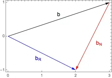
The vector $\color{blue}{b_{\mathcal{R}}}$ is projection of the data vector $b$ onto $\color{blue}{\mathcal{R}(\mathbf{A})}$. Pick a vector in the span,
$$
\color{blue}{s} =
\color{blue}{\left[
\begin{array}{r}
2 \\
-1
\end{array}
\right]}
$$
Compute the solution vector
$$
\color{blue}{b_{\mathcal{R}}}
=
b \cdot
\frac{\color{blue}{s}}{\lVert \color{blue}{s} \rVert}
=
\color{blue}{
\left[
\begin{array}{r}
2 \\
-1
\end{array}
\right]}
$$
Solve the consistent linear system
With a data vector in the range space, the linear system is now consistent and can be solved with Gaussian-Jordan Elimination.
$$
\begin{array}{ccc}
\left[
\begin{array}{c|c}
\mathbf{A} & \color{blue}{b_{\mathcal{R}}}
\end{array}
\right]
& \to &
\left[
\begin{array}{c|c}
\mathbf{E_{A}} & R
\end{array}
\right]
\\
\left[
\begin{array}{rrr|r}
2 & -2 & 4 & 2 \\
-1 & 1 & -2 & -1\\
\end{array}
\right]
& \to &
\left[
\begin{array}{rrr|r}
1 & -1 & 2 & 1 \\
0 & 0 & 0 & 0\\
\end{array}
\right]
\end{array}
$$
Craft solution
The interpretation of the reduced matrix $\mathbf{E_{A}}$ is
$$
x - y + 2z = 1.
$$
To match the convention posed in the question, let
$$ y = s, \quad z = t$$ to recover
$$
x = s -2t + 1, \qquad s,t \in \mathbb{R}.
$$
The least squares minimizes are the set
$$
\boxed{
x_{LS} =
\left[
\begin{array}{c}
s - 2t + 1 \\
s \\
t
\end{array}
\right]}.
$$
This represents the complete set of minimizers without resolving the range and null space components $\color{blue}{x_{p}} + \color{red}{x_{h}}.$
To connect the pieces, note that the values $s=-\tfrac{1}{6}$, $t=\tfrac{1}{3}$ produce $\color{blue}{x_{p}}$.
Solution via normal equations
The normal equations will not produce a particular solution, but they will provide the set of least squares minimizers.
The product matrix is singular:
$$
\begin{array}{ccc}
\mathbf{A}^{*}\mathbf{A} x
& = &
\mathbf{A}^{*} b
\\
\left[
\begin{array}{rrr}
5 & -5 & 10 \\
-5 & 5 & -10 \\
10 & -10 & 20 \\
\end{array}
\right]
& = &
\left[
\begin{array}{rrr|r}
5 \\
-5 \\
10
\end{array}
\right]
\end{array}
$$
Because rank$\left(\mathbf{A}\right) = 1$, the product matrix is also rank 1 and offers no inverse. The usual solution path
$$
\color{blue}{x_{p}} = \left( \mathbf{A}^{*}\mathbf{A}\right)^{-1}
\mathbf{A}^{*} b
$$
is not available.
However, Gauss-Jordan elimination of the normal equations produces
$$
\begin{array}{ccc}
\left[
\begin{array}{c|c}
\mathbf{A}^{*}\mathbf{A} & \mathbf{A}^{*} b
\end{array}
\right]
& \to &
\left[
\begin{array}{c|c}
\mathbf{E_{A}} & R
\end{array}
\right]
\\
\left[
\begin{array}{rrr|r}
5 & -5 & 10 & 5 \\
-5 & 5 & -10 & -5 \\
10 & -10 & 20 & -10 \\
\end{array}
\right]
& \to &
\left[
\begin{array}{rrr|r}
1 & -1 & 2 & 1 \\
0 & 0 & 0 & 0\\
0 & 0 & 0 & 0\\
\end{array}
\right]
\end{array}
$$
This is the same result from the previous solution.
Solution via singular value decomposition
The SVD will provide the pseudoinverse matrix needed by $\color(blue){x_{p}}$ and the null space projector for $\color(red){x_{h}}$.
For derivations, refer to
How does the SVD solve the least squares problem?.
General solution for the least squares problem
The general solution for the least squares problem in $(1)$ is
$$
x_{LS} = \color{blue}{x_{p}} + \color{red}{x_{h}} = \underbrace{\mathbf{A}^{\dagger}b\vphantom{\big|}}_{\color{blue}{x_{p}}} +
\underbrace{\left( \mathbf{I}_{n} - \mathbf{A}^{\dagger} \mathbf{A}\right) y}_{\color{red}{x_{h}}}, \qquad y\in\mathbb{R}^{n}
$$
Singular value decomposition form
The form of the singular value decomposition for this rank deficient problem is
$$
\begin{align}
\mathbf{A} &= \mathbf{U} \, \Sigma \, \mathbf{V}^{*}
=
% U
\left[ \begin{array}{cc}
\color{blue}{\mathbf{U}_{\mathcal{R}(\mathbf{A})}} & \color{red}{\mathbf{U}_{\mathcal{N}(\mathbf{A}^{*})}}
\end{array} \right]
% Sigma
\left[ \begin{array}{cc}
\mathbf{S} & \mathbf{0} \\
\mathbf{0} & \mathbf{0}
\end{array} \right]
% V
\left[ \begin{array}{l}
\color{blue}{\mathbf{V}_{\mathcal{R}(\mathbf{A}^{*})}^{*}} \\
\color{red}{\mathbf{V}_{\mathcal{N}(\mathbf{A})}^{*}}
\end{array} \right]
\end{align}
$$
Moore-Penrose pseudoinverse matrix form
The corresponding Moore-Penrose pseudoinverse matrix is
$$
\begin{align}
%%
\mathbf{A}^{\dagger} &= \mathbf{V} \, \Sigma^{\dagger} \, \mathbf{U}^{*}
=
% U
\left[ \begin{array}{cc}
\color{blue}{\mathbf{V}_{\mathcal{R}(\mathbf{A}^{*})}} &
\color{red}{\mathbf{V}_{\mathcal{N}(\mathbf{A})}}
\end{array} \right]
% Sigma
\left[ \begin{array}{cc}
\mathbf{S}^{-1} & \mathbf{0} \\
\mathbf{0} & \mathbf{0}
\end{array} \right]
% V
\left[ \begin{array}{l}
\color{blue}{\mathbf{U}_{\mathcal{R}(\mathbf{A})}^{*}} \\
\color{red}{\mathbf{U}_{\mathcal{N}(\mathbf{A}^{*})}^{*}}
\end{array} \right]
\end{align}
$$
Computing the SVD
Computational details can be found in Computing the SVD, and examples in Calculating SVD by hand: resolving sign ambiguities in the range vectors., and, Need to multiply by -1 for a SVD to work?.
Singular value spectrum
The first step is to compute the singular values, which are the square roots of the ordered, non-zero, eigenvalues to the product matrix: $$\mathbf{A}\mathbf{A}^{*} = 6
\left[
\begin{array}{rr}
4 & -2 \\
-2 & 1 \\
\end{array}
\right].$$
Pulling out the scaling factor of $6$ is not required, it's a personal peccadillo to simply hand calculations. Proceeding, the characteristic polynomial for the scaled eigenvalues $\Lambda$ is
$$
p(\Lambda) = \det
\left[
\begin{array}{rr}
4-\Lambda & -2 \\
-2 & 1-\Lambda \\
\end{array}
\right]
=
\Lambda(\Lambda - 5)
$$
The scaled and ordered eigenvalue spectrum is
$$
\Lambda \left( \mathbf{A}\mathbf{A}^{*} \right) = \left\{ 5, 0\right\}
$$
Restore the original scale of the eigenvalues using $\lambda = 6 \Lambda$, and take the square root:
$$
\sigma = \sqrt{\lambda} = \sqrt{30}.
$$
Resolve$\ \color{blue}{\mathbf{V}_{\mathcal{R}}}$
As there is but one vector in the domain,
$$
\color{blue}{\mathbf{V_{\mathcal{R}}}} = \frac{1}{6}
\color{blue}{\left[
\begin{array}{r}
1 \\
-1 \\
2
\end{array}
\right]}
$$
Resolve$\ \color{blue}{\mathbf{U_{\mathcal{R}}}}$
The final step is
$$
\color{blue}{\mathbf{U_{\mathcal{R}}}} = \frac{1}{\sigma}\mathbf{A} \color{blue}{\mathbf{V}_{\mathcal{R}}} =
\frac{1}{\sqrt{5}}
\color{blue}{\left[
\begin{array}{r}
-2 \\
1
\end{array}
\right]}
$$
Assemble the Moore-Penrose pseudoinverse matrix
Using the thin SVD, the pseudoinverse matrix is
$$
\mathbf{A}^{\dagger} = \frac{1}{30}
\left[
\begin{array}{r}
2 & -1\\
-2 & 1\\
4 & -2
\end{array}
\right].
$$
Particular solution
The particular solution is the least squares solution of least norm and is computed using the pseudoinverse matrix:
$$\color{blue}{x_{p}} = \mathbf{A}^{\dagger} b = \frac{1}{6}
\color{blue}{
\left[
\begin{array}{r}
1 \\
-1 \\
2
\end{array}
\right]
}, $$
as expected.
Homogeneous solution
Assemble the projector onto $\ \color{red}{\mathcal{N} \left( \mathbf{A} \right)}$
The homogeneous term is handled by the projector onto $\color{red}{\mathcal{N} \left( \mathbf{A} \right)} $. Start with the projector onto the range space $\color{blue}{\mathcal{R} \left( \mathbf{A}^{*} \right)}$:
$$
\mathbf{P}_{\color{blue}{\mathcal{R} \left( \mathbf{A}^{*} \right)}} = \frac{1}{6}
\left[
\begin{array}{rrc}
1 & -1 & 2 \\
-1 & 1 & 2 \\
2 & -2 & 4 \\
\end{array}
\right]
$$
The projector needed for the least squares solution is the projector onto the orthogonal complement of $\color{blue}{\mathcal{R} \left( \mathbf{A}^{*} \right)}$: the projector onto the null space $\color{red}{\mathcal{N} \left( \mathbf{A} \right)}$. This projector is
$$
\mathbf{P}_{\color{red}{\mathcal{N} \left( \mathbf{A} \right)}} =
\mathbf{I}_{3} - \mathbf{P}_{\color{blue}{\mathcal{R} \left( \mathbf{A}^{*} \right)}}
$$
Final solution
Using the SVD, the least squares solution set is given by
$$
\boxed{
x_{LS} = \color{blue}{x_{p}} + \color{red}{x_{h}} =
%%
\mathbf{A}^{\dagger}b +
\left( \mathbf{I}_{n} - \mathbf{A}^{\dagger} \mathbf{A}\right) y
=
\frac{1}{6}
\color{blue}{
\left[
\begin{array}{r}
1 \\
-1 \\
2
\end{array}
\right]}
+
\frac{1}{6}
\left[
\begin{array}{rcr}
5 & 1 & -2 \\
1 & 5 & 2\\
-2 & 2 & 2
\end{array}
\right]y
, \qquad y\in\mathbb{R}^{n}}
$$

