Regular polygon inside another?

Question

Inspired by this question, I was wondering if one can generalize to the case of an $n$-gon.

For example, when $n=5$ we have this picture:

where $ABCDE$ is a regular pentagon, $AA_1=BB_1=\cdots=EE_1$. Also $A,A_1,B_1$ are colinear in that order, and so on.

Can we conclude that $A_1B_1C_1D_1E_1$ is regular? Or is there a counterexample for that?

Answer 1

Update

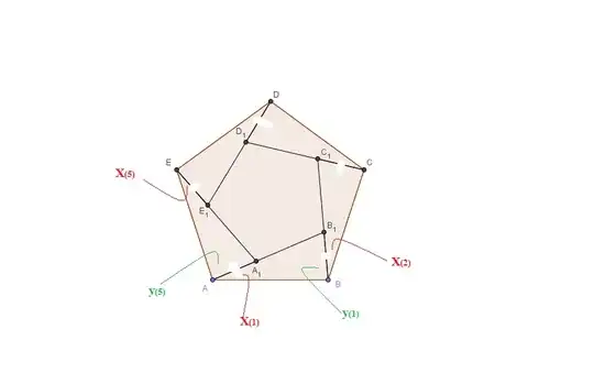
Won't include the trig as rather lengthy, but included as visual complement to give genreal idea:

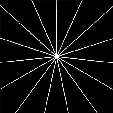
Note that a shutter on a traditional camera works on this same principal:

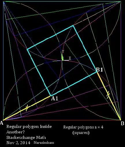
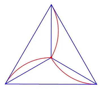
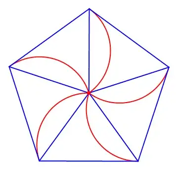
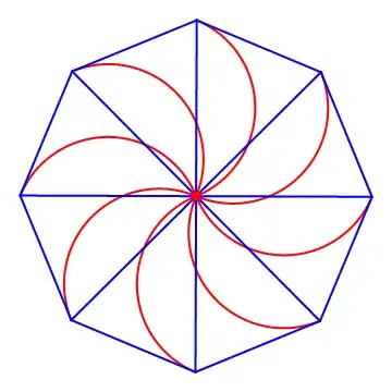
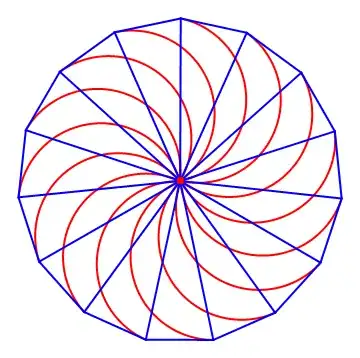
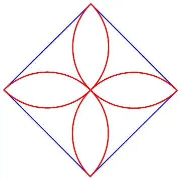
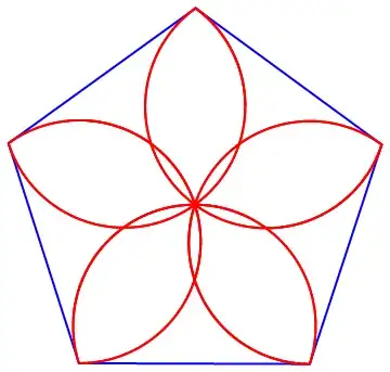
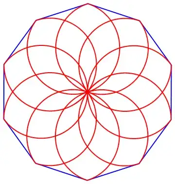
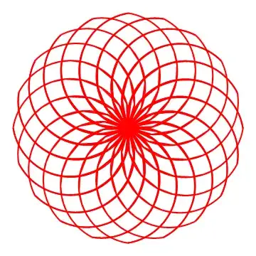
Note also that Narasimham's observation of the paths taken offer visual proof of the conjecture, and for greater $n$, are quite visually compelling:

Related

---

Code at Narasimham's request:

Manipulate[
Show[\[Theta] = LambertW[1]//N; length = -10; g = 0.2; 
tt = {1.337, 1.236, 1.18, 1.144, 1.121, 1.104, 1.091, 1.081, 1.073, 
1.066, 1.061, 1.056, 1.052, 1.049, 1.046, 1.043, 1.041, 1.039};
r = c*(rr = 
  If[n < 2*Pi, 
   Pi + n*(-1 + 2*Pi) + 
    n*ArcTan[
      Cos[1] + Cos[1 - (4*Pi)/n] + 2*Cos[1 - (2*Pi)/n] - 
       2*Sqrt[2]*
        Sqrt[(3 + Cos[(2*Pi)/n])*Sin[Pi/n]^2*Sin[1 - (2*Pi)/n]^2],
       4*Cos[Pi/n]^2*Sin[1 - (2*Pi)/n] + 
       2*Sqrt[2]*Cot[1 - (2*Pi)/n]*
        Sqrt[(3 + Cos[(2*Pi)/n])*Sin[Pi/n]^2*
          Sin[1 - (2*Pi)/n]^2]], 
   Pi + n*(-1 + 2*Pi) + 
    n*ArcTan[
      Cos[1] + Cos[1 - (4*Pi)/n] + 2*Cos[1 - (2*Pi)/n] + 
       2*Sqrt[2]*
        Sqrt[(3 + Cos[(2*Pi)/n])*Sin[Pi/n]^2*Sin[1 - (2*Pi)/n]^2],
       4*Cos[Pi/n]^2*Sin[1 - (2*Pi)/n] - 
       2*Sqrt[2]*Cot[1 - (2*Pi)/n]*
        Sqrt[(3 + Cos[(2*Pi)/n])*Sin[Pi/n]^2*
          Sin[1 - (2*Pi)/n]^2]]]);
 aa = Table[{Cos[1 + (2*k*Pi)/n]*Cos[\[Theta]] - 
  Sin[1 + (2*k*Pi)/n]*Sin[\[Theta]], 
 Cos[\[Theta]]*Sin[1 + (2*k*Pi)/n] + 
  Cos[1 + (2*k*Pi)/n]*Sin[\[Theta]]}, {k, Join[{n}, Range[n]]}]; 
 li = Table[{(2*
    Sin[r/n]*(-Sin[1 + ((2*s + 1)*Pi)/n + \[Theta]] + 
      Cos[Pi/n]*Sin[(n + (2*s + 1)*Pi + r + n*\[Theta])/n]))/(3 + 
    Cos[Pi/n]^2 - 4*Cos[Pi/n]*Cos[r/n] - 
    Sin[Pi/n]^2), (2*(Cos[1 + ((2*s + 1)*Pi)/n + \[Theta]] - 
      Cos[Pi/n]*Cos[(n + (2*s + 1)*Pi + r + n*\[Theta])/n])*
    Sin[r/n])/(3 + Cos[Pi/n]^2 - 4*Cos[Pi/n]*Cos[r/n] - 
    Sin[Pi/n]^2)}, {s, 1, n}]; 
 list = Join[Drop[li, n - 2], Take[li, n - 2]];
 Graphics[{Opacity[If[TrueQ[JamesBond] == True, 1, 0]], Black, 
 Polygon[{{-(1 + g), -(1 + g)}, {1 + g, -(1 + g)}, {1 + g, 
   1 + g}, {-(1 + g), 1 + g}}], {Red, Thick, 
 Opacity[If[TrueQ[JamesBond] == True, 0, 
   If[TrueQ[circles] == True, 1, 0]]], Circle[]}, {Red, Thick, 
 Opacity[If[TrueQ[JamesBond] == True, 0, 
   If[TrueQ[circles] == True, 1, 0]]], Circle[{0, 0}, Cos[Pi/n]]},
 Opacity[If[TrueQ[JamesBond] == True, 0, 1]], Thick, Blue, 
Line[aa], Opacity[If[TrueQ[JamesBond] == True, 1, 0]], White, 
Polygon[list], Opacity[1], 
If[TrueQ[JamesBond] == True, White, Blue], Thick, 
bb = Table[Line[{aa[[u]], list[[u]]}], {u, 1, n}], 
Opacity[If[TrueQ[JamesBond] == True, 0, 1]], Red, 
PointSize[Large], Point[list], 
If[TrueQ[JamesBond] == True, White, Red], 
Opacity[If[TrueQ[JamesBond] == True, 1, 
  If[TrueQ[lines] == True, 1, 0]]], 
Table[Line[{bb[[u, 1, 
    1]], {bb[[u, 1, 2, 
      1]] + ((bb[[u, 1, 2, 1]] - bb[[u, 1, 1, 1]])*length)/
      Sqrt[Abs[(bb[[u, 1, 1, 1]] - 
            bb[[u, 1, 1, 2]])*2 + (bb[[u, 1, 1, 2]] - 
            bb[[u, 1, 2, 2]])*2]], 
    bb[[u, 1, 2, 
      2]] + ((bb[[u, 1, 2, 2]] - bb[[u, 1, 1, 2]])*length)/
      Sqrt[Abs[(bb[[u, 1, 1, 1]] - 
            bb[[u, 1, 1, 2]])*2 + (bb[[u, 1, 1, 2]] - 
            bb[[u, 1, 2, 2]])*2]]}}], {u, 1, n}]}], 
 PlotRange -> {{-(1 + g), 1 + g}, {-(1 + g), 1 + g}}], {{c, 
 If[TrueQ[min] == True, 1.18, 1]}, 
If[TrueQ[min] == True, Evaluate[tt[[n - 2]]], 1],
Dynamic[
1*n*(Pi/If[n < 2*Pi, 
   Pi + n*(-1 + 2*Pi) + 
    n*ArcTan[
      Cos[1] + Cos[1 - (4*Pi)/n] + 2*Cos[1 - (2*Pi)/n] - 

       2*Sqrt[2]*
        Sqrt[(3 + Cos[(2*Pi)/n])*Sin[Pi/n]^2*Sin[1 - (2*Pi)/n]^2],
       4*Cos[Pi/n]^2*Sin[1 - (2*Pi)/n] + 
       2*Sqrt[2]*Cot[1 - (2*Pi)/n]*
        Sqrt[(3 + Cos[(2*Pi)/n])*Sin[Pi/n]^2*
          Sin[1 - (2*Pi)/n]^2]], 
   Pi + n*(-1 + 2*Pi) + 
    n*ArcTan[
      Cos[1] + Cos[1 - (4*Pi)/n] + 2*Cos[1 - (2*Pi)/n] + 
       2*Sqrt[2]*
        Sqrt[(3 + Cos[(2*Pi)/n])*Sin[Pi/n]^2*Sin[1 - (2*Pi)/n]^2],
       4*Cos[Pi/n]^2*Sin[1 - (2*Pi)/n] - 
       2*Sqrt[2]*Cot[1 - (2*Pi)/n]*
        Sqrt[(3 + Cos[(2*Pi)/n])*Sin[Pi/n]^2*
          Sin[1 - (2*Pi)/n]^2]]])]}, {{n, 5}, 3, 20, 
 1}, {{circles, False}, {True, False}}, {{lines, False}, {True, 
 False}}, {{JamesBond, False}, {True, False}}, {{min, False}, {True,  False}}]

paths calculated separately with

n = 10;
Show[\[Theta] = LambertW[1]//N;
aa = Table[{Cos[1 + (2 k \[Pi])/n] Cos[\[Theta]] - 
 Sin[1 + (2 k \[Pi])/n] Sin[\[Theta]], 
Cos[\[Theta]] Sin[1 + (2 k \[Pi])/n] + 
 Cos[1 + (2 k \[Pi])/n] Sin[\[Theta]]}, {k, Join[{n}, Range[n]]}];

Graphics[{Thick, Blue, Line[aa]}], Show[\[Theta] = LambertW[1];

 Graphics[Thick, Blue, Line[aa]], 
  r = c*(Pi + 20*(-1 + 2*Pi) + 
  20*ArcTan[(4*Cos[Pi/20]^2*Sin[1 - Pi/10] - 
       2*Sqrt[2*(3 + Sqrt[5/8 + Sqrt[5]/8])]*Cos[1 - Pi/10]*
        Sin[Pi/20])/(Cos[1] + Cos[1 - Pi/5] + 2*Cos[1 - Pi/10] + 
       2*Sqrt[2*(3 + Sqrt[5/8 + Sqrt[5]/8])]*Sin[1 - Pi/10]*
        Sin[Pi/20])]);

  Table[ParametricPlot[\[Theta] = LambertW[1]//N; {(
  2 Sin[r/n] (-Sin[1 + ((2 s + 1) \[Pi])/n + \[Theta]] + 
    Cos[\[Pi]/n] Sin[(n + (2 s + 1) \[Pi] + r + n \[Theta])/n]))/(
  3 + Cos[\[Pi]/n]^2 - 4 Cos[\[Pi]/n] Cos[r/n] - Sin[\[Pi]/n]^2), (
  2 (Cos[1 + ((2 s + 1) \[Pi])/n + \[Theta]] - 
    Cos[\[Pi]/n] Cos[(n + (2 s + 1) \[Pi] + r + n \[Theta])/
      n]) Sin[r/n])/(
  3 + Cos[\[Pi]/n]^2 - 4 Cos[\[Pi]/n] Cos[r/n] - 
  Sin[\[Pi]/n]^2)}, {c, 0, 0.5}, Axes -> False, PlotRange -> All, 
  PlotStyle -> {Red, Thick}], {s, 1, n}]]]

just change n as desired.

---

Original answer

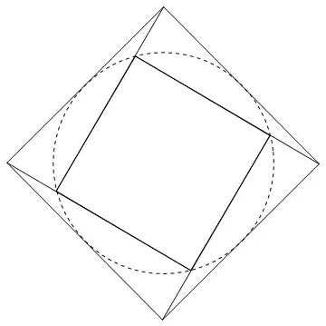
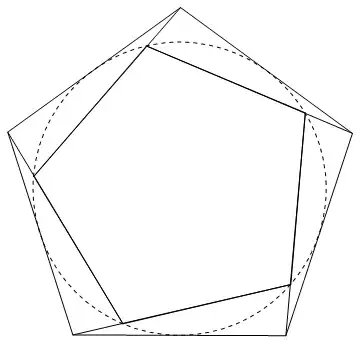
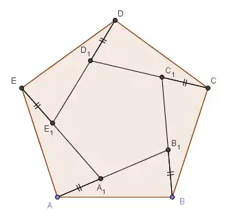
Idea

Since all regular polygons can be inscribed in the unit circle, a circle can then be inscribed in the polygon (dashed) and a further polygon inside that. If lines then join the vertices of the outer polygon to the corresponding ones of the inner polygon, the outer polygon can be fixed while the inner is rotated. The adjoining lines will then form a third polygon that decreases in size to $0$ when the inner polygon is rotated a half turn. Since the outer is fixed, the relation follows.

Details

A polygon inscribed in a unit circle has vertices at $$e^{i(1 + 2\pi k/n)}$$ for all $k=1$ to $n$, where $n$ is the number of sides of the polygon. This can be described in cartesian coordinates as $$\{\Re\ e^{i(1 + 2\pi k/n)},\Im\ e^{i(1 + 2\pi k/n)}\}.$$ The polygon can then be rotated about the origin so that the uppermost vertex lies on the $y$-axis by multiplying by matrix

\begin{pmatrix} \Re \ e^{i\Omega} & -\Im \ e^{i\Omega}\\ \Im \ e^{i\Omega}& \Re \ e^{i\Omega}\\ \end{pmatrix}

where $\Omega$ is the Omega constant.

A smaller circle, with radius $\Re \ e^{i\pi/n}$, where $n$ is the number of sides of the polygon, can then be inscribed inside it.

The polygon to be inscribed and rotated within that will then have coordinates

\begin{align} \Re \ e^{i\pi/n} \begin{pmatrix} \Re \ e^{i\Omega_{1}} & -\Im \ e^{i\Omega_{1}}\\ \Im \ e^{i\Omega_{1}}& \Re \ e^{i\Omega_{1}}\\ \end{pmatrix} \cdot \{\Re\ e^{i(1 + 2\pi k/n)},\Im\ e^{i(1 + 2\pi k/n)}\} \end{align}

where $\Omega_{1}=\dfrac{r}{n}+\Omega$, with $r$ ranging from $0$ to $n\pi.$

---

Mathematica code to play with:

Manipulate[ Show[\[Theta] = LambertW[1] // N; 
c = Re[E^( I Pi/n)]; \[CapitalTheta] = r/n + \[Theta]; 
Graphics[{(*Circle[]*){Circle[{0, 0}, c]}, 
Line[aa = (Table[{{Re[E^( I \[Theta])], -Im[E^( I \[Theta])]}, 
{Im[E^( I \[Theta])], Re[E^( I \[Theta])]}}.{Re[ E^(I  (1 + 2 \[Pi] k/n))], 
Im[E^(I (1 + 2 \[Pi] k/n))]}, {k, Join[{n}, Range[n]]}])],
Line[bb = (c Table[{{Re[E^( I \[CapitalTheta])], -Im[E^( I \[CapitalTheta])]}, 
{Im[E^( I \[CapitalTheta])], 
Re[E^( I \[CapitalTheta])]}}.{ Re[E^(I ( 1 + 2 \[Pi]  k/n))], 
Im[E^(I ( 1 + 2 \[Pi]  k/n))]}, {k,Join[{n}, Range[n]]}])], 
Line[Table[{aa[[q]], bb[[q]]}, {q, 1, n}]] }], Axes -> False, 
PlotRange -> {{-1, 1}, {-1, 1}}], {{r, 0}, 0, n Pi}, {{n, 3}, 3, 20, 1}]

Answer 2

1. Let's begin our discussion by setting $\angle AEE_1$ as $\alpha$, $|AA_1|=d$, and generalizing for an arbitrary perfect polygon, $\gamma$ as the angle $\angle EAB$ (which is of course $\pi(\frac{n-2}n)$ radians for an n-sided polygon), and for simplicity set $|AB|=1$.

2. Draw a perpendicular line to $EA_1$ from A. Assume for now that the intersection point is actually on $EA_1$ and not an extension (we'll get back to this point later). Mark the intersection point as $F$, and mark $\angle FAA_1 = \beta$. We then have $|AF| = \sin \alpha$ and $d \cos \beta = \sin \alpha$, and let's define function $f$ as the resulting angle: $\angle BAB_1 = f(\alpha) = \gamma - \beta - \frac {\pi}{2} + \alpha$.

3. Naturally in the trivial solution $f(\alpha) = \alpha$, which means for example for 5 sides $\beta = \pi / 10$.

4. Now suppose $f(\alpha) > \alpha$. We get $$\gamma - \beta - \frac {\pi}{2} + \alpha > \alpha$$ $$\gamma - \frac {\pi}2 - \arccos(\frac{\sin \alpha}d) > 0$$ However because $f(\alpha) > \alpha$, and because both angles are acute (if $\alpha$ is not acute, $AA_1$ is opposite the largest angle in triangle $AA_1E$, which would make $|AA_1| > |EA_1| > |EE_1|$ which is a contradiction. The same argument works for $f(\alpha) < \frac {\pi}2$), $\sin(f(\alpha)) > \sin(\alpha)$.

5. Because $\arccos$ is a monotonous decreasing function $$\arccos(\frac{\sin(f(\alpha))}d) < \arccos(\frac{\sin(\alpha)}d)$$. Therefore: $$f(f(\alpha)) = \gamma - \frac {\pi}2 - \arccos(\frac{\sin f(\alpha)}d) + f(\alpha) > \gamma - \frac {\pi}2 - \arccos(\frac{\sin \alpha}d) + f(\alpha) > f(\alpha)$$

6. Switching the signs in the inequalities, the same argument demonstrates that if $f(\alpha) < \alpha$ then $f(f(\alpha)) < f(\alpha)$. Meaning that repeating $f$ is either monotonous decreasing, increasing or constant (in the trivial solution).

7. But remember that if we repeat the function $f$ n-times we must get $\alpha$ again! This is because $f$ just calculates the next angle while going around the $n$-sided polygon, and after $n$ steps we just return to the original starting point. For example, in the 5-sided polygon we must have $f(f(f(f(f(\alpha)))) = \alpha$. But this is impossible if the composition of the functions is strictly increasing or decreasing.

8. Therefore $f(\alpha) = \alpha$ for all $n$-sided regular polygons, all the triangles in the drawing are congruent and the internal polygon must be regular as well.

9. Now we return to explaining why point $F$ must be on the line $EA_1$ and not on its extension. If this was possible, then the angle $\angle BAB_1$ would be $g(\alpha) = \gamma - \frac{\pi}2 + \beta + \alpha$ (notice the sign change before $\beta$ as opposed to $f(\alpha)$). Composition of $g$ is obviously monotonously increasing because $g(\alpha) > \alpha$.

10. Let's mark $\delta(d) = \arcsin(d \cos(\gamma - \frac{\pi}2))$. If $\alpha > \delta(d)$, it is easy to see $f(\alpha) > \alpha$. This means that for $\alpha > \delta(d)$ both $g(\alpha) > \alpha$ and $f(\alpha) > \alpha$. Therefore we note that if $\alpha > \delta(d)$ no sequence of compositions of $f$ and $g$ can equal to $\alpha$.

11. So if we show $g(\alpha) > \delta(d)$ for all $\frac{\pi}2 > \alpha > 0$, we know that no sequence of compositions over $g(\alpha)$ would be ever equal to $\alpha$.

12. $$g(\alpha) = \gamma - \frac{\pi}2 + \arccos(\frac{\sin(\alpha)}d) + \alpha \ge \frac{\pi}2 - \arcsin(\frac{\sin(\alpha)}d) + \alpha$$ This inequality holds for $n > 3$ which was already proven in the original question. We'll now show: $$ \alpha + \frac{\pi}2 \ge \arcsin(\frac{\sin(\alpha)}d) + \delta(d)$$ But we know $\delta(d) \le \arcsin(d)$ because $\arcsin$ is strictly increasing, so if we prove $ \alpha + \frac{\pi}2 \ge \arcsin(\frac{\sin(\alpha)}d) + \arcsin(d)$ we proved our inequality.

13. $$\frac{d}{d\alpha}(\arcsin(\frac{\sin(\alpha)}d) + \arcsin(d) - \alpha) = \frac{\cos \alpha}{d \sqrt{1 - \frac{\sin ^2 \alpha}{d^2}}} - 1 \ge 0$$ The last inequality is true because $\cos \alpha > d$ (because $|EA_1| > |EE_1| = |AA_1|$). Therefore $\arcsin(\frac{\sin(\alpha)}d) + \arcsin(d) - \alpha$ is strictly increasing, and the maximal value would be $\alpha = \arcsin(d)$ (the function is undefined for higher $\alpha$). But $$ \arcsin(\frac{\sin(\alpha)}d) + \arcsin(d) - \alpha = \arcsin(1) = \frac{\pi}2 $$

14. Therefore we conclude $$ \alpha + \frac{\pi}2 \ge \arcsin(\frac{\sin(\alpha)}d) + \arcsin(d) \ge \arcsin(\frac{\sin(\alpha)}d) + \delta(d) $$ hence $$g(\alpha) \ge \frac{\pi}2 - \arcsin(\frac{\sin(\alpha)}d) + \alpha \ge \delta(d)$$

15. Finally, we conclude that any sequence of composition of $f$ and $g$ than includes at least one $g$ must become monotonously increasing, and therefore the only solution to the problem is the one using only $f$ (and so $F$ is on the line $EA_1$). QED.

Answer 3

Very interesting geometric puzzle. It is true or valid for any regular polygon of n sides.Continuously changing side $AB_1$ of shrinking side polygon $A_1B_1$ rotated in the manner indicated. Rotated polygons have different size but are all regular.

EDIT2:

$AA_1B_1$ is a given straight line. The sum of all external angles $ n AB_1B$ is $ 2\pi$ for any polygon in one single rotation of $AB$,so each angle $ AB_1B$ is given as $ 2 \pi/n $ for a regular polygon due to cyclic symmetry.

Moreover, a straight line $ x \,cos \alpha + y \,sin \alpha = p $ becomes $ x \, cos (\alpha+\beta) + y \,sin (\alpha+\beta) = p $ by rotation through $\beta $, leaving external $ AB_1B$ invariant around regular polygon.

EDIT1:

Took previous ABC equilateral triangle case for inspiration only. An independent problem circumstance/statement as I have taken/assumed taken is:

Lines AB,... of a regular polygon are rotated about regular polygon corner A by equal angles $B_1 A B$,... so that intercepts $ A A_1, B B_1 $ are of equal length. Show that the enclosed reduced polygon is also regular.

Logic of method is recognizing locus containing $B_1$ is a circular arc. By Law of Sines $ AB / sin (2 \pi/n) = BB_1/ sin (B_1 A B)$ = constant suggests that polygon corner has a locus on a circle passing through A and B. The locus of A and B are circular arcs with polar offset $ 2 \pi/ n $.

It is proved that all surmises are quite correct. (Collinearity, regular polygon similarity upto side length or size, difference of $ AB_1$ and $B_1B $ being the side of rotating polygon etc.) while staying on this arc.

As the corner goes to center of arc polygon gets smaller, but extension of sides go through the vertices of un-rotated polygon!

To visualize this, construct a circle of radius $ a/( 2 sin( \pi/n))$ through $A$ and $B$. Draw two rays through polygon corner B1, mark left side by removing right side length $ B_1B $ at left ray and draw a circle through $A B_1 B$. complete construction of polygon. ( For higher n compass /ruler construction is not known, only n = 17 done by KF Gauss.). One can construct by finding chords and marking off corners.

Repeat the construction for several positions of corner point to visualize successively reducing regular polygons.

I have sketched squares in n = 4 case. Constructions of pentagons, hexagons are likewise possible, with more time.

Would be fun on Java Sketch Pad or similar dynamic geometric animation to see changing polygon positions go through one set of extended bases of polygon to fixed polygon corners/vertices. Enclosing extensions would make the setup look like the iris or light arresting diaphragm of a lens in a camera..

Incidentally the problem can also be stated like this in other words:

n-fold symmetry Polygon Iris: Between two fixed points$ A$ and $B$ a point $B_1$ is moving on a circular arc of radius $ a/( 2 sin( \pi/n))$ such that difference of $ AB_1$ and $B_1B = A_1B_1$ forms a regular n-polygon side. Show that all polygon extensions pass through vertices of regular n-polygon with this difference $ A_1B_1$ as side.

Answer 4

I think it is true.

The construction (and hence the proof) will be easier to start with inclined angle instead of length.

Starting from $A$, the ray $AB_1$ is drawn inclining at angle $x_1$ to the adjacent side $AB$. Then the ray $BC_1$ with $x_2 = x_1$. The process is continued until $EA_1$ is formed.

Note that all x’s are equal. Therefore all y’s are also equal because the polygon is regular.

Then, $⊿ABB_1$ is congruent to $⊿BCC_1$ …… (ASA)

Therefore, $BB_1 = CC_1 = …$.

This further means $A_1B_1 = B_1C_1 = ….$, implying that the constructed polygon is also regular.