6

Update

The polynomials are generated as follows:

Where

$B_n(x) = \sum_{k=0}^n {n \choose k} b_{n-k} x^k$

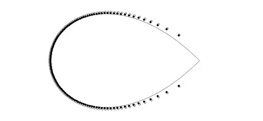
is used to generate standard Bernoulli polynomials, top plot is generated as follows:

$B_n^{(1)}(x) = -\sum_{k=0}^n {n \choose k} |\Re(b^{(1)}_{n-k})+ \Im(b^{(1)}_{n-k})| x^k$

using definition of $b^{(1)}_{n}$ as outlined below.

(Note: Where $b^{(1)}_{1}={\tilde{\infty}}$, substitute for usual $-\frac{1}{2}$.)

The second plot is exactly the same as above except that the first term of $B_n^{(1)}(x)$ has a positive value.

Original question

Since

$\zeta(2n) = (-1)^{n+1} \, \frac{2^{2n-1} \, b_{2n} \, \pi^{2n}}{(2n)!},\quad n \ge 0, \,$

where $b_{2n}$ are the Bernoulli numbers, rearranging & substituting $2n$ for $n$, we get:

$b_{n}^{(1)} = \frac{\zeta(n)\, n!}{(-1)^{\frac{n}{2}+1} \, 2^{n-1} \, \pi^{n}}$

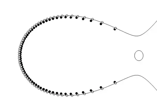
Using $b_{n}^{(1)}$ to generate a series similar to the usual Bernoulli polynomials (the main difference being that the odd real $b_{n}$ are give complex values rather than 0), the roots of $B_{n}^{(1)}(x)$ differ from the usual pattern of the $B_{n}(x)$ roots and fit a scaled Szegő Curve even more tightly (bar a couple of spare roots off the diagram) than the roots of the partial sums of $e^x$ (white, outlined points):

enter image description here

Another curious modfication, with roots plotted against scaled Szegő Curve, circle (radius $\frac{n}{e}$) & roots of $e^x - 1$ (white, outlined points):

enter image description here

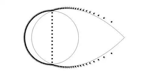
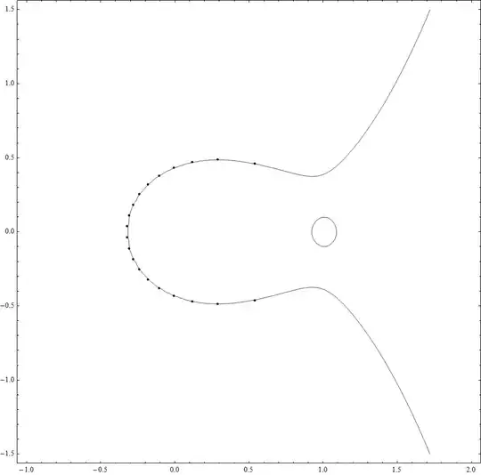
Image of the two root plots against a dynamic Szegő Curve, as given by Antonio Vargas' code below (included for comparison purposes).

enter image description here

Despite fairly extensive searches on the internet, I have found no literature on the subject. I was wondering if anyone knew of any?

martin
  • 8,998
  • To clarify, do you mean $$B_n^{(1)}(x) = -\sum_{k=0}^n {n \choose k} \left|b^{(1)}_{n-k}\right| x^k$$ ? And when you say that for the second plot the first term of $B_n^{(1)}(x)$ has a positive value, what does it have in the first plot? – Antonio Vargas Nov 07 '13 at 02:27
  • Yes, thanks for that correction - but forgot to mention that only real & imaginary parts are taken to generate polynomials. Please see edited update. So all values are negative for top plot, and all are negative for bottom plot, except for first term. Hope I've been a little clearer, and haven't made too many mistakes! – martin Nov 07 '13 at 03:03
  • To clarify, the first plot shows the roots of the following polynomial:

    $$B_n^{(1)}(x) = -\sum_{k=0}^n {n \choose k} |\Re(b^{(1)}{n-k})+ \Im(b^{(1)}{n-k})| x^k$$

    $$where$$

    $$b_{n}^{(1)} = \frac{\zeta(n), n!}{(-1)^{\frac{n}{2}+1} , 2^{n-1} , \pi^{n}},$$

    $$and$$

    $$b^{(1)}_{1}=-\frac{1}{2}$$

    – martin Nov 07 '13 at 03:23

1 Answers1

1

There are some possibilities which could explain the behavior you notice, but I'm just making guesses based on related phenomena. Proving any of this is likely difficult.

Just as the usual Bernoulli polynomials approximate the sine and cosine (see, e.g., Theorem 1 in this paper), your polynomials may approximate the exponential function. In fact they may approximate the partial sums of the exponential function in some sense, which could explain the behavior of their zeros.

I gave some references for the zeros of the usual Bernoulli polynomials which may be enlightening in this answer.

If I understand correctly, you are considering the zeros of $B_n^{(1)}(x) + \text{const.}$ in the second plot. This mirrors the behavior of the zeros of the partial sums of the exponential function $s_n[\exp](z)$. The zeros of $s_n[\exp](nz)$ converge to the usual Szegő curve, and the zeros of $s_n[\exp](z) + \text{const.}$ converge to the Szegő curve in the right half plane and to the circle $|z| = 1/e$ in the left half plane. The zeros on the imaginary axis approximate the zeros of $e^{nz} + \text{const.}$

See, for example, this question on MathOverflow.

This is very much related to the fact that $e^{nz} + c \sim e^{nz}$ for $\Re(z) > 0$ and $e^{nz} + c \sim c$ for $\Re(z) < 0$, though I'm not sure what the link would be to your case.


Below is some Mathematica code to plot the intermediate Szegő curves for the exponential function as mentioned in the comments.

s[n_, z_] := Sum[z^k/k!, {k, 0, n}];  
m = 20;  
Show[  
    ContourPlot[  
        Abs[(x+I y) E^(1-x-I y)]^m == Sqrt[2 Pi m] Abs[(1-x-I y)/(x+I y)],  
        {x, -1, 2}, {y, -3/2, 3/2}],  
    ListPlot[
        {Re[z], Im[z]} /. NSolve[s[m, m z] == 0, z],  
        PlotStyle -> Black]  
]

This produces the output

enter image description here

  • There are a couple of points off the plot (on the negative real line), which bother me slightly! Would they have any bearing on the closeness of the approximation of the polynomial to the exponential function? – martin Nov 07 '13 at 03:32
  • 1
    It's hard to say. It appears that they each tend to a limit as $n \to \infty$, so it might be the case that your polynomials approximate $p(x)e^{x}$, where $p(x)$ is some polynomial whose zeros are those limit points. – Antonio Vargas Nov 07 '13 at 03:59
  • Wow! Just plotted $e^x - 1$ after looking at the MathOverflow link you provided & very close to second plot (now edited to include circle & roots of $e^x - 1$). - Many thanks for your help on this - you have raised many interesting points for me. – martin Nov 07 '13 at 10:55
  • I'm glad you found the answer helpful :). – Antonio Vargas Nov 07 '13 at 11:49
  • 1
    Also, I suggest you try plotting the roots of $B_n^{(1)}\left(\frac{n}{2\pi} x\right)$ as well; this is the proper scaling to have the zeros accumulate on the usual Szegő curve $|ze^{1-z}| = 1$. – Antonio Vargas Nov 07 '13 at 11:51
  • OK, thanks - yes, I came at it from the other side! :) – martin Nov 07 '13 at 14:28
  • One question I do have, is do you know how I would go about plotting the dynamic Szegő curves as on page 4 of this paper: http://www.math.ucla.edu/~dupuy/notes/partialsums.pdf ? – martin Nov 07 '13 at 14:38
  • 1
    Ah sure, I've seen that paper. I think there is a typo in the definition of those Dynamic Szegő curves $D_n$. The original definition can be found in this paper (pdf) in equation $(1.6)$. You'll notice there's this quantity $\tau_n$ there; you can ignore this and get approximately the same curve (they differ by at most $O(1/n^2)$). I'll edit my answer to include some mathematica code to plot the dynamic Szegő curves. – Antonio Vargas Nov 07 '13 at 15:21
  • Thank you so much for your help on this - especially the mathematica code, it really is very much appreciated :) ... Another interesting paper by Carpenter & Varga: http://www.math.kent.edu/~varga/pub/paper_233.pdf – martin Nov 07 '13 at 16:43