Here's my asymptotic approach:
Let consider the (equivalent, as pointed out by Henry) case of strong compositions of $n+k=m$ into $k$ positive parts.
In probabilistic terms, we have $k$ random variables $x_i$ taking values on $1\cdots m$,
with $\sum x_i =m$ and were all the possible realizations are equiprobable.
I claim (if my life does not depend on it) that that problem is asymptotically equivalent (why? in what sense? explained below) to having
$k$ iid geometric random variables $y_i$ (taking values on $1\cdots \infty$) with mean $m/k=1/p$ (notice that here $\sum y_i$ is not fixed, but $E[\sum y_i] =m$).
Then, a first approximation would be
$\displaystyle E_M = E(max(x_i)) -1 \approx E(max(y_i)) -1 = G\left(k,\frac{k}{k+n}\right) - 1$
where $G(k,p)$ is the expectation of the maximum of $k$ IID geometric random variables of parameter $p$. This later problem is discussed here and here. The exact formula is rather complicated:
$\displaystyle G(k,p) = \sum_{i=1}^k \binom{k}{i} (-1)^{i+1} \frac{1}{1-(1-p)^i}$
A tight approximation is given by:
$\displaystyle G(k,p) \approx \frac{H_k}{- \log(1-p)} + \frac{1}{2} $ , with $\displaystyle H_k=\sum_{i=1}^k \frac{1}{i}$ (harmonic number).
what gives our second approximation:
$\displaystyle E_M \approx \frac{H_k}{\log(1+k/n)} - \frac{1}{2}$
And for $n$ increasing with $k$ constant, the first order expansion of the logarithm
gives this third approximation, which shows the linear increasing observed by Henry:
$\displaystyle E_M \approx n \frac{ H_k} {k} - \frac{1}{2} \approx n \frac{ H_k} {k}$ $ \hspace{14pt} (n \to \infty)$
It is also readily seen that if both $n,k$ increase with constant ratio, then $E_M$ grows as $\log(k)$.
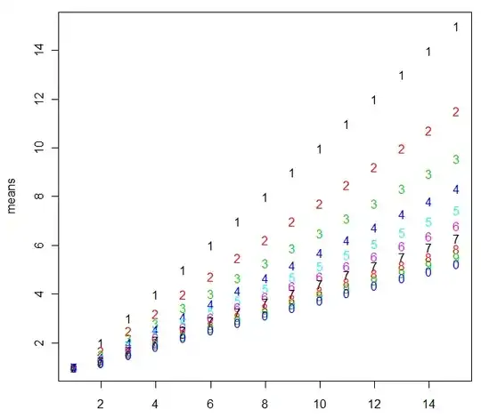
Some results, for comparing with Henry's values, for the second approximation (very similar to the first one; the third one is quite more coarse)
         1      2      3      4      5      6      7      8      9     10
  1  0.9427 0.8654 0.8225 0.7944 0.7744 0.7591 0.7469 0.7370 0.7286 0.7215
  2  1.9663 1.6640 1.5008 1.3963 1.3226 1.2673 1.2239 1.1887 1.1595 1.1347
  3  2.9761 2.4364 2.1449 1.9588 1.8280 1.7301 1.6536 1.5918 1.5407 1.4975
  4  3.9814 3.1995 2.7761 2.5056 2.3157 2.1738 2.0631 1.9739 1.9002 1.8380
  5  4.9848 3.9580 3.4007 3.0444 2.7942 2.6073 2.4617 2.3444 2.2476 2.1661
  6  5.9872 4.7141 4.0216 3.5784 3.2670 3.0346 2.8535 2.7077 2.5874 2.4862
  7  6.9889 5.4686 4.6401 4.1093 3.7363 3.4577 3.2407 3.0661 2.9221 2.8010
  8  7.9902 6.2221 5.2570 4.6381 4.2030 3.8780 3.6248 3.4210 3.2531 3.1119
  9  8.9912 6.9749 5.8728 5.1655 4.6679 4.2962 4.0065 3.7734 3.5813 3.4198
 10  9.9921 7.7272 6.4877 5.6917 5.1314 4.7127 4.3864 4.1239 3.9075 3.7256
 11  10.9927 8.4791 7.1021 6.2171 5.5939 5.1281 4.7649 4.4728 4.2320 4.0296
 12  11.9933 9.2307 7.7159 6.7418 6.0555 5.5424 5.1424 4.8205 4.5552 4.3322
 13  12.9938 9.9821 8.3294 7.2660 6.5165 5.9560 5.5189 5.1672 4.8773 4.6336
 14  13.9943 10.7333 8.9426 7.7897 6.9770 6.3690 5.8948 5.5132 5.1985 4.9341
 15  14.9946 11.4844 9.5555 8.3132 7.4370 6.7814 6.2700 5.8584 5.5190 5.2338
Some (loose) justification about the aproximation. For those who are familiar with statistical
physics, this is much related with a hard-rod (unidimensional) gas, over a discrete space,
with the distance between consecutive particules as variables, and the (asympotical)
equivalence of two "ensembles": the original has fixed volume (m) and number of particles (k)
(that would correspond to a "canonical" ensemble), the second keeps the number of particles
but the volume is allowed to vary (would be an isobaric ensemble), but such that the mean
volume is equal to the fixed volume of the original. The condition that the configurations
of the original ensemble have equal probability is related to a system with no interaction
energy (except for the exlusion), and that corresponds (in the second ensemble) to a
particle that can appear at each cell with a probability independent of its neighbours: and from here I got the geometrical.
In other terms, the equivalence might be justified in that the second probalistic model
is equal to the first if conditioned on the event that the variables sum up to $m$ -
and asymptotically we are less likely to depart from this case.
All this does not provide a rigorous proof, of course. One could also object that this
kind of approximation by "ensemble equivalence" is plausible for computing the typical
statistical magnitudes that are mostly related to averages - but here we are computing
extreme value, it's less clear that it must work.
Added: Some clarification about the aproximation method:
Recall that ${\bf x}=\{x_i\}$ , $i=1\cdots k$ is our original discrete random variable; it support is restricted by $x_i\ge 1$ and $\sum x_i = m= n+k$. Inside this region, all realizations has equal probability, so the probability function is constant:
$P({\bf x}) = \frac{1}{Z}$
( $Z(n,k)$, the "partition function", would be the count of all possible configurations, but that does not matter here).
On the other side, the proposed ${\bf y}=\{y_i\}$ has iid geometric components, with parameter $p=k/m$, so its probability function is
$\displaystyle P({\bf y}) = \prod p (1-p)^{y_i} = p^k (1-p)^{\sum y_i}$
with $y_i \ge 1$. Calling $ s({\bf y})=\sum y_i$, it is readily seen that if we condition on $s = m$, we get the original distribution (it's constant, and in the same region).
$P({\bf y} | s = m ) = P({\bf x})$
We are interested in $E[g({ \bf x})]$, where $g({\bf x}) = max(x_1 \cdots x_k)$, and want to see if it can be approximated by $E[g({\bf y})]$ (some loose notation here)
$\displaystyle E[g({\bf y})] = \int g({\bf y}) P({\bf y}) dy = \int g({\bf y}) \sum_s P({\bf y} | s) P(s) dy $
Now, because the way we choose $p$, we have $E(s)=m$, and we can expect that $P(s)$ will be highly peaked around that value (to show that the statistical ensembles -canonnical, microcanonical, grand-canonical, etc- are asympotically equivalent, one uses this line of reasoning ). And so, asympotically, we can expect to be justified in aproximate the sum by that single term. What would mean that
$E[g({\bf y})] \approx E[g({\bf x})]$