1

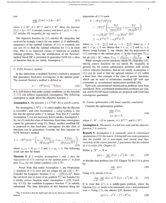
In the arcticle Fixed-Time Stable Gradient Flows: Applications to Continuous-Time Optimization I found an interesting formula and its properties. The screenshot of the page from the article I was led below.

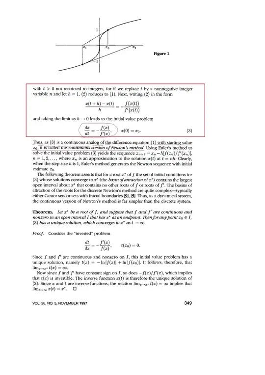
In another article A Continuous Version of Newton's Method, I found a similar formula, but in contrast to the first article, where the ratio of the gradient $G$ to the hessian $H$ is used, i.e. $G/H$, this use $f(x)/G(x)$. Screenshot from the article I also led below.

Problem: I decided to "play" with formula

$\frac{dx}{dt}=-(\frac{d^2f}{d^2x})^{-1}\frac{df}{dx}$

and function $f(x)$

$f(x)=e^{-(x-x_*)^2}$

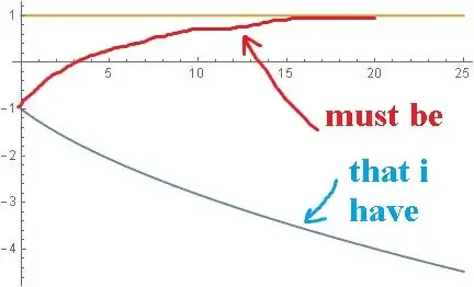
and found that none of them work as it should (you need convergence from the starting point $x(0)$ to the point $x_*$).

Below I give code from Mathematica and what happened.

Clear["Derivative"]

ClearAll["Global`*"]

pars = {xstart = -1, xend = 1}

f = Exp[-(x[t] - xend)^2]

E^-(-1 + x[t])^2

sys = NDSolve[{x'[t] == -(D[D[f, x[t]], x[t]])^-1 D[f, x[t]], x[0] == xstart}, {x}, {t, 0, 500}]

Plot[{Evaluate[x[t] /. sys], xend}, {t, 0, 25}, PlotRange -> Full, PlotPoints -> 100]

enter image description here

Question: What's wrong with this formula or where did I make a mistake?

I will be glad any help.
enter image description here

enter image description here

dtn
  • 731
  • 1
  • 6
  • 19

1 Answers1

1

In the screenshoted page, theorem 3 ensures convergence to the optimal point $x_*$ in fixed time if assumptions 1 and 3 are satisfied.

Assumption 1 (not on the screenshot) ask for the optimal value $x_*$ ($f(x_*)$ is the minimum of $f$) to be reached at finite values. However, since you took $f(x)=e^{-(x-x_*)^2}$, $f(x_*)=1$ is actually the maximum and the minimum of the function, $0$ is reached at $\pm \infty$ (explaining why your solution seems to decrease to $-\infty$).

Considering $f(x)=-e^{-(x-x_*)^2}$ instead should do the trick if the initial point is close enough to $x_*$ for the assumptions of the theorem to be verified (this function is strictly convex only near it and this is required by assumption 3).

nicomezi
  • 8,254
  • You're right. I noticed that the selection of the sign before the function does not play a special role. The initial point plays a much larger role. This is especially noticeable if you look at the function gradient. The trajectory "falls" there, where it is more convenient to fall, and not where it is necessary. And can we somehow correct this problem? – dtn Apr 10 '21 at 06:24
  • 1
    With the toy function we are considering here, the problem is that the derivative quickly becomes close to $0$ if we get too far from $x_$. With strict convexity (assumption 3) and minimum reached somewhere (assumption 1), you ensure that the derivative will never get arbitrarily close to $0$ when you are far from $x_$. I hope this helps. – nicomezi Apr 10 '21 at 06:33
  • If you are interested, pay attention to the article. I worked on it in the morning, I wanted to reproduce the results, but I did not work. I unlikely somewhere wrong, it seems to me that the mistake is in the article itself.

    https://www.sciencedirect.com/science/article/abs/pii/s0005109812002324

    – dtn Apr 10 '21 at 07:02
  • 1
    The article is pretty dense, is there a specific part where you are particularly suspicious about it ? – nicomezi Apr 12 '21 at 06:05
  • The main problems are two:
    1. The settlement of the convergence time (18) and the time defined through numerical analysis give different results.
    2. When changing the function, the system is unstable or not in the extremum (depends on the choice of parameters).

    It is impossible to add this approach to genral. A truly generalized system should converge in extremum from anywhere. Consideration of it as a locally corresponding quadratic this in my opinion is too hard assumption.

    – dtn Apr 12 '21 at 06:25
  • In attempts to understand obvious and sharply throwing into the eyes of some errors, I did not meet. At first, I suggested that the function does not meet the condition of Polyak-Lojasiewicz (5) on the explicit convexity and placed the starting point closer to the extremum. The results did not give it. Then I drew attention to formulas (24b) and (27). They are present at $1/\epsilon_2$ and $(2 \pi)/\epsilon_2$ relations, which provided (for $\epsilon_2 << 1$ the enormous values ​​of these coefficients. – dtn Apr 12 '21 at 06:28
  • This may be the cause of instability. I replaced them with the coefficients less and found that with some values, the system is stable, but it loses the convergence property for the final time, or "freezes" in one position. Determine the ranges of performance is almost unrealistic. In general, it would be wonderful if this article tried to reproduce the expert. I did the code in Mathematica. – dtn Apr 12 '21 at 06:29
  • 1
    Thank you. I am sorry to tell you this but I think the appropriate way would be to write another question. This way it is more likely for you to have an answer. I will try to have a deeper look at it. – nicomezi Apr 12 '21 at 06:40
  • https://math.stackexchange.com/questions/4114416/finite-time-criterion-for-ode – dtn Apr 24 '21 at 06:10