Comment: You can get a reasonable approximation to $Var(\alpha)$ by simulation. In the simulation, I assume
the 51 numbers are selected without replacement.
set.seed(2020)
alpha = replicate(10^5, sum(sample(1:159, 51)))
summary(alpha)
   Min. 1st Qu.  Median    Mean 3rd Qu.    Max.
   2915    3897    4081    4081    4266    5275
Notice that among the 100,000 samples I summed, all of the totals
are between the two numbers you mention in your question.
var(alpha)
[1] 74069.39
sd(alpha)
[1] 272.1569
A histogram of the simulated values of $\alpha$ looks approximately normal, so I show the best-fitting normal
density along wit the histogram.
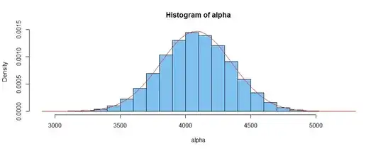
hist(alpha, prob=T, col="skyblue2")
 curve(dnorm(x, mean(alpha), sd(alpha)), add=T, col="red")
With replacement, the variance is somewhat larger.
(Again here the distribution of $\alpha$ seems approximately normal; histogram not shown.)
set.seed(1130)
alpha = replicate(10^6, sum(sample(1:159, 51, rep=T)))
summary(alpha)
   Min. 1st Qu.  Median    Mean 3rd Qu.    Max.
   2593    3859    4080    4080    4302    5590
var(alpha)
[1] 107274.7
Possible solution: If you consider the population to be numbers 1 through 159, then the population has variance 2120, and the sum of a random sample with replacement should have variance 51 times as large, which is 108,120, which seems to agree with the simulated result within the margin of simulation error.
var(1:159)
[1] 2120
51*var(1:159)
[1] 108120
