Rank comparison for different low rank approximations

Question

I want to approximate a correlation matrix by low-rank components such that $$\Sigma \approx \sum_{i=1}^{k_1} \sigma_ib_ib_i^T$$

where $\Sigma$ is of size $n \times n$, $b$ is a $n$ dimensional vector and $k$ is the number of components. I was wondering if subtracting a diagonal matrix $D \in R^{n\times n}$ from the matrix would give a better low rank approximation, below is the decomposition

$$\Sigma \approx D + \sum_{i=1}^{k_2} \sigma_{i}^{'} b_{i}^{'}b_i^{'T}$$

Can we estimate $D, \sigma, b$ such that $k_2 \leq k_1$ holds true? Both the above approximations have different $\sigma$ and $b$.

Also, I know that the $\Sigma$ matrix has non-zero diagonal entries and the matrix after removing the diagonal term is sparse.

Edit 1: I was thinking of simulating correlation matrix and then test the above hypothesis. Is there is a way to simulate a low rank, sparse and full diagonal matrix? I have asked this question here https://stats.stackexchange.com/questions/368868/simulation-of-low-rank-and-sparse-matrix

Answer 1

The Eckart Young Mirsky Theorem States the following. Suppose $A \in \mathbb{R}^{m \times n}$

$$ A = U \Sigma V^{T} \tag{1} $$

then if we take a rank k approximation of the matrix using the SVD

$$A_{k} = \sum_{i=1}^{k} \sigma_{i}u_{i}v_{i}^{t} \tag{2} $$

the difference between them is given as

$$ \| A - A_{k} \|_{2} = \bigg\| \sum_{i=k+1}^{n} \sigma_{i}u_{i} v_{i}^{t} \bigg\| = \sigma_{k+1} \tag{3}$$

The best rank k approximation is when the matrix has the given rank k. This is from this expression. If $A= A_{k}$ our minimization expression will be minimized.

I am not sure how $D$ is going to help you better approximate the matrix $\Sigma $. I am sorry about the confusion with notation.

Right, if $k_{2}$ is less than $k$ it is actually not good

$$ \| A + D\| \leq \| A \| + \|D\| \tag{4}$$

and we can approximate both of these. The norm is

$$ \| A\|_{2} = \sqrt{\lambda_{max}(A^{*}A)} = \sigma_{max}(A) = \sigma_{1} \tag{5}$$

the 2-norm is the maximum singular value. $$ \| A + D\| \leq \sigma_{max}(A) + \sigma_{max}(D) \tag{6}$$

So from above, you have

$$ \| A -\Sigma_{1} \|_{2} = \sigma_{k_{1}+1} \tag{7} $$ $$ \| A- \Sigma_{2} \|_{2} - \|D \|_{2} \leq \| A - \Sigma_{2} -D \|_{2}\tag{8} $$ Then

$$ \| A- \Sigma_{2}\|_{2} = \sigma_{k_{2}+1} \\ \|D\|_{2} = \sigma_{max}(D) \tag{9}$$

$$ \sigma_{k_{1}+1} - \sigma_{k_{2}+1} - \sigma_{max}(D) \leq \|A-\Sigma_{1} \|_{2} -\|A-\Sigma_{2} -D\|_{2} \tag{10}$$

Note that singular values are ordered so $\sigma_{k_{1}+1} \geq \sigma_{k_{2}+1}$ if $k_{1} \geq k_{2}$

Numerical Simulation

I think you wanted a numerical simulation to support your argument so I am going to create the Python code to show you why. I already answered a similar question about SVDs earlier. So I will use that code to show you.

Say we have our covariance matrix or really any matrix $A$ and it has a rank $\alpha$,

import numpy as np
import matplotlib.pyplot as plt
import math



def gen_rank_k(m,n,k):
# Generates a rank k matrix
# Input m: dimension of matrix
# Input n: dimension of matrix
# Input k: rank of matrix

    vec1 = np.random.rand(m,k)
    vec2 = np.random.rand(k,n)
    rank_k_matrix = np.dot(vec1,vec2)

    return rank_k_matrix

m=10
n=m
alpha = 7

A = gen_rank_k(m,n,k)

Now we have $k_{2} \leq k_{1} \leq \alpha $

u, s, vh = np.linalg.svd(A, full_matrices = False)

x = np.linspace(1,10,10)

plt.plot(x,s)

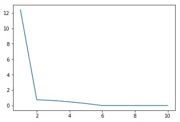
This is a plot of the singular values of $A$

now for the two low rank approximations of $A$ choose $k_{1} = 5, k_{2} = 3$

def low_rank_k(u,s,vh,num):
# rank k approx

    u = u[:,:num]
    vh = vh[:num,:]
    s = s[:num]
    s = np.diag(s)
    my_low_rank = np.dot(np.dot(u,s),vh)
    return my_low_rank

my_rank_k1 = low_rank_k(u,s,vh,k1)
my_rank_k2 = low_rank_k(u,s,vh,k2)

my_diagonal_matrix  = np.diag(np.random.rand(10))

error1 = np.linalg.norm(A - my_rank_k1)
error2 = np.linalg.norm(A- my_rank_k2 - my_diagonal_matrix)