How to apply SVD to real data to reduce the number of parameters?

Question

I have a question about applying the Singular Value Decomposition (SVD) to real data. Say I have the equation $$ y= Ax+v$$ where $A \in \mathbb{R}^{m \times n}$, $y \in \mathbb{R}^m$, $x \in \mathbb{R}^n$, and $v \in \mathbb{R}^m$ is the noise. And I want to estimate $x$, which are the parameters connecting measurements in $A$ to observations in $y$.

Let’s say I discover that my matrix $A$ has about 20 singular values which are significant, and then after that the singular values are miniscule (i.e. very small and insignificant). And the matrix $A$ is $m=300k, n=10k$ so I have 300k observations in the vector $y$.

From what I understand, this means the following:

• Even though I can still construct the $300k$ observations in $y$ from the $A$ matrix, it has many measurements which don’t contribute much, so those should be removed.
• To fix this either:
  • Take SVD of the matrix $A,$ and only use the most significant parameters, i.e. the most significant 20. This will slim down the A matrix and make it more skinny (reduce the number of columns in $A$).
  • Take more observations in a different, independent way, in addition to the 300k. This will add rows to the $A$ matrix, and will add values to the $y$ vector. See if it increase the number of significant singular values. If so, take more measurements in that different, independent way.

My question is: If my understanding above is correct, then how will knowing which singular values are significant, tell me which parameters to keep, and which ones to throw away? If I want to make the matrix $A$ skinnier and not use all 10k columns, then how do I know which columns correspond to the 20 most significant singular values?

This example was taken from about 62 minutes into Lecture 17 the Stanford course https://see.stanford.edu/Course/EE263/56 .

Answer 1

Typically you wouldn't be able to use a personal computer for that. The size of the matrix is enormous. I am going to ignore the fact you typically care about the data. So people would typically use the PCA or something.

General Formulation of the Problem

In general, the SVD is the following.

$$ A = U \Sigma V^{T} \tag{1}$$

right, where $UU^{T} = U^{T}U = I_{m} $ , $ VV^{T} = V^{T}V = I_{n} $ are orthogonal. The singular values are actually given in descending order. That is

$$ \sigma_{1} \geq \sigma_{2} \geq \cdots \geq \sigma_{n} > 0 \tag{2} $$

If you have the following equation

$$ y = Ax+v \tag{3}$$

we can say

$$ y- v = Ax \implies U\Sigma V^{T}x = y-v \tag{4} $$

Now this simply turns into

$$ x = V \Sigma^{-1} U^{T}(y-v) \tag{5} $$

Ok...right. If we want to apply a low rank approximation of $U \Sigma V^{T}$ we are simply choosing the $k$ largest singular values like the following.

$$ A_{k} = \sum_{i=1}^{k} \sigma_{i} u_{i} v_{i}^{t} \tag{6} $$

$$ A_{k} = U_{m \times k} \Sigma_{k \times k} V_{k \times n}^{T} \tag{7}$$

Note when take the inverse of $ \Sigma$ it is simply a diagonal matrix so we

$$ \Sigma^{-1} \implies \frac{1}{\sigma_{i}} \tag{8} $$

Now we may not know the amount of noise in the signal. There are actually techniques for this. I think it is called Tikhonov Regularization. So you can introduce a regularization parameter $\lambda $.

I don't think I actually addressed how you would know. If you can do the following. Say take $k$ singular values and form a low rank approximation like above and the original matrix. We get this equation.

$$ \| A - A_{k} \|_{2} = \bigg\| \sum_{i=k+1}^{n} \sigma_{i} u_{i} v_{i}^{t}\bigg\|_{2} = \sigma_{k+1} \tag{9} $$

If the $\sigma_{k+1} $ is relatively small for you then you may be happy.

In terms of real world data this doesn't really hold what happens when you apply the SVD. You'd have to look into the principal components analysis. That is if you are thinking that first 20 columns are still: red, blue, length of hair. They aren't. They are linear combinations that are orthogonalized. The data transformations are called the principal components.

Tikhonov Regularization looks like this

$$ \hat{x} = \min_{x} \| y- Ax \|_{2}^{2} + \|\Gamma x \|_{2}^{2} \tag{10}$$

where $ \Gamma$ is a matrix

For your questions

Even though I can still construct the 300k observations in y from the A matrix, it has many measurements which don’t contribute much, so those should be removed.

This is correct. There is likely some relationship you could come up with between the data and your measurements but adding more measurements wouldn't do any good. This is an area of research called inverse problem theory.

If I want to make the matrix A skinnier and not use all 10k columns, then how do I know which columns correspond to the 20 most significant singular values?

Where the SVD comes from

Part of the problem with the SVD is what it does. If you just want to look at this from the minimizing error aspect you can use the SVD. The principal component analysis is another method which is the statiscal cousin of the SVD. One way of understanding this is actually understanding how the SVD is computed. If I have a data matrix $A$ then the SVD is the actually formed from the eigendecomposition of the covariance matrix $A^{T}A$

$$ A^{T}A = (U \Sigma V^{T})^{T} U \Sigma V^{T} \tag{11}$$

$$ A^{T}A = V \Sigma^{T} U^{T} U \Sigma V^{T} \tag{12}$$

using orthogonality

$ U^{T}U = UU^{T} = I_{m} $

$$ A^{T}A = V \Sigma^{T} \Sigma V^{T} \tag{13}$$

also we know

$ \Sigma^{T} \Sigma = \Sigma \Sigma^{T} = \Lambda $

$$ A^{T}A = V \Lambda V^{T} \tag{14}$$

Similarly

$$ AA^{T} = U \Lambda U^{T} \tag{15}$$

Low rank Approximation

I think there was some trouble understanding what it means to make a low-rank approximation. I can do this fairly easily. Say we construct a matrix randomly in Python that is rank-deficient.

import numpy as np
import matplotlib.pyplot as plt
m=10
n=m
k=5


def gen_rank_k(m,n,k):
# Generates a rank k matrix
# Input m: dimension of matrix
# Input n: dimension of matrix
# Input k: rank of matrix

    vec1 = np.random.rand(m,k)
    vec2 = np.random.rand(k,n)
    rank_k_matrix = np.dot(vec1,vec2)

    return rank_k_matrix

A = gen_rank_k(m,n,k)
u, s, vh = np.linalg.svd(A, full_matrices = False)

x = np.linspace(1,10,10)

plt.plot(x,s)

my_rank = np.linalg.matrix_rank(A)

If you wanted to visualize the singular values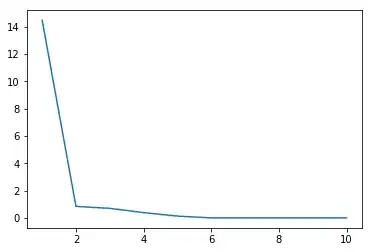

Note our command above..

my_rank = np.linalg.matrix_rank(A)

my_rank
Out[9]: 5

how do you choose them? You can do it fairly simply like this.

def low_rank_k(u,s,vh,num):
# rank k approx

    u = u[:,:num]
    vh = vh[:num,:]
    s = s[:num]
    s = np.diag(s)
    my_low_rank = np.dot(np.dot(u,s),vh)
    return my_low_rank

This part here is

$$ A_{k} = U_{m \times k} \Sigma_{k \times k} V_{k \times n}^{T} \tag{16}$$

my_rank_k = low_rank_k(u,s,vh,5)

my_error = np.linalg.norm(A-my_rank_k)

This part is

$$ \| A - A_{k} \|_{2} = \bigg\| \sum_{i=k+1}^{n} \sigma_{i} u_{i} v_{i}^{t}\bigg\|_{2} = \sigma_{k+1} \tag{17} $$

my_error
Out[7]: 6.541665918732523e-15

now if you look $k=5$ what is $\sigma_{k+1} = \sigma_{6}$

s[6]
Out[6]: 3.8119202900864143e-16

Some other visuals

There is some other visuals for a reduced SVD versus a full SVD

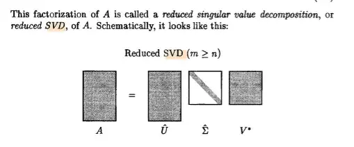
if you note that section there is all $0$. The interpretation is you form these $20$ components $U\Sigma$ . The coefficients in the vectors tell you how much of each predictor you are using and the singular values $\sigma$ are telling you the magnitude in the direction of the orthogonal component it goes. Visually like above.

If you look at these singular values they decay.

Creating Pseudo Inverse

Technically to generate the pseudo inverse $A^{\dagger}$ we should do the following. The $\sigma_{i}$ past the rank are going to blow up because they are not $0$

Choose parameter $\epsilon$. Now we can form the matrix $\Sigma^{\dagger}$ like this.

$$ \Sigma^{\dagger} =\begin{align}\begin{cases} \frac{1}{\sigma_{i}} & \sigma_{i} \leq \epsilon \\ 0 & \sigma_{i} > \epsilon \end{cases} \end{align} \tag{18}$$

Which gives us

$$A^{\dagger} = V \Sigma^{\dagger} U^{T} \tag{19} $$