Expected time till absorption in specific state of a Markov chain

Question

This question is a follow-up to Expected number of steps for reaching a specific absorbing state in an absorbing Markov chain because I don't understand the answer given there. I think I need to see a concrete example.

Suppose I play red and black at a casino. On each play, I either win the amount I staked, with probability $p<\frac12$ or I lose my stake. Let's say I start with a bankroll of $2$ and I decide to play until I have won $3$ or lost everything. My strategy is to bet just enough to reach my goal, or everything I have, whichever is less.

We have a Markov chain with $6$ states, $2$ of which are absorbing. There are well-known methods to determine the probability of winning, and of determining the average number of plays I make, but what if I want to know the average number of plays I make if I reach my goal? The transition matrix, with $q=1-p$ is $$\begin {bmatrix} 1&0&0&0&0&0\\ q&0&p&0&0&0\\ q&0&0&0&p&0\\ 0&q&0&0&0&p\\ 0&0&0&q&0&p\\ 0&0&0&0&0&1 \end{bmatrix}$$

Henning Malcolm suggests two approaches, neither of which I can follow. (This is because of my limitations, and is in no way intended as a criticism of the answer.) The first assumes that I have figured out the probability of winning starting with every possible bankroll. Then we are to compute new transition probabilities that describe the experience of the winners, as I understand it, and compute the time to absorption in the new chain. Let $p_k$ be the probability of winning, if my bankroll is $k$. How should I calculate the new transition matrix?

Henning Malcolm gives an alternative method if there is only one starting state we're interested in, and I'm only interested in the actual case where I start in state $2$. He says, "first set up a system of equations that compute for each state the expected number of times one will encounter that state before being absorbed." If we let $e_k$ be this number for state $k=1,2,3,4,$ how do we construct the equations relating the $e_k?$ I can see how to do this if we only care about the number plays until the game ends, but how do I make it reflect only the number of plays until winning?

Answer 1

$\color{red}{\textbf{The currently accepted answer (as of 2022-12-16) is incorrect.}}$ Here I'll give an example that makes the incorrectness clear. Then I'll provide a correct method to solve this problem, including examples and a Mathematica implementation.

Paraphrasing the other answer

Let $X$ denote the number of steps until absorption, and let $Z_j$ be the event "we end up in absorbing state $S_j$." ($Z_j$ is only meaningful for $j$ s.t. $S_j$ is an absorbing state.) Suppose we want $E[X | Z_G]$ for some goal state $S_G$. The other answer suggests the following algorithm:

1. Delete the other absorbing state state(s) from the system.
2. Iteratively delete any state that can only transition to deleted state(s). Repeat until there's an iteration with no new deletions.
3. For each state that currently could transition to one or more deleted states, modify its transition probabilities to condition on not transitioning to those deleted states on the current step.
4. The above steps give a modified Markov chain in which every transient state eventually ends up at $S_G$. Use standard methods to find $E[X]$ for that MC. This is the answer to the original problem.

Why that answer is incorrect (example)

First, an example. Let's say we have states $S_0, S_1, S_2, S_3$ which represent my current bankroll. If I have \$0 I can't play anymore. If I have \$1, I bet my dollar on a coin toss with $P[\text{win}] = \frac 1 {1000}$, ending up with either \$0 or \$2. If I have \$2, I bet \$1 on a coin toss with $P[\text{win}] = \frac 1 2$, ending up with either \$1 or \$3. Finally, if I have \$3 then I go home happy.

The transition matrix is: $$P = \left(\begin{array}{cccc} 1 & 0 & 0 & 0 \\ \frac{999}{1000} & 0 & \frac{1}{1000} & 0 \\ 0 & \frac{1}{2} & 0 & \frac{1}{2} \\ 0 & 0 & 0 & 1 \end{array} \right)$$

Let's say I start the game with \$2 and I want to compute $E[S | Z_3]$. If I follow the algorithm described above, I will first delete the other absorbing state $S_0$, then adjust the transition probabilities from $S_1$, getting the new matrix $$\hat P = \left(\begin{array}{ccc} 0 & 1 & 0 \\ \frac{1}{2} & 0 & \frac{1}{2} \\ 0 & 0 & 1 \end{array} \right)$$

At this point we can find the expected absorption time by Markov chain methods, or even just in our heads because the new MC is so simple. I'll demo the second approach just for fun. We have $\frac 1 2$ chance to win in 1 step, then $\frac{1}{4}$ chance to win in 2 steps, then $\frac{1}{8}$ chance to win in 3 steps, and so on, so the expected game length is $$E[X | Z_3] = \sum_{n=1}^\infty \frac{n}{2^n} = \color{red}{\boxed{2}}.$$

This answer doesn't pass intuitive sanity checks. Think back to the original Markov chain before we pruned it. We have $\frac{1}{2}$ chance of winning the game on the first turn. If we don't win immediately, then we move to state $S_1$, and from there we have extremely high probability of losing the game immediately. This means that the games where we win will overwhelmingly be games where we just won the very first coin toss, so we should get $E[X | Z_3] = 1 + \varepsilon$ where $\varepsilon$ is some TBD small positive number. I'll use this same example below and we can confirm this intuition.

Corrected algorithm

We can follow these steps:

1. For each state $S_j$, compute $g_j := P[Z_G | \text{ start at } S_j]$. There's a standard formula to compute these; see Wikipedia.
2. Now compute a whole new transition matrix $\tilde P$. If $p_{jk}$ was the original transition probability from $S_k$ to $S_j$, then define $\tilde p_{jk} = P[\text{step from $S_k$ to $S_j$} | Z_G]$. This can be computed using Bayes' Theorem and it turns out we get $\tilde p_{jk} = \frac{g_j p_{jk}}{g_k}$; see extra details below. Exception: We don't modify the transition probabilities starting from absorbing states.
3. The modified Markov chain $\tilde P$ exactly describes the transition probabilities for random walkers who will eventually end up state $S_G$ (unless they started in some other absorbing state). The expected time till absorption in this MC is exactly the quantity we set out to find, and we can compute it using another standard MC method.

Step (2) is not on Wikipedia's list of standard MC calculations, so I'll give extra details here. The idea is to use Bayes' Theorem but with all probabilities conditioned on our current location being $S_k$. We compute: $$\begin{align} \tilde p_{jk} &= P[\text{next location is $S_j$} | Z_G, \text{current location is $S_k$}] \\ &= \frac{P[Z_G | \text{next location is $S_j$, curr location is $S_k$}] P[\text{next location is $S_j$ | curr location is $S_k$}]}{P[Z_G | \text{curr location is $S_k$}]} \\ &= \frac{g_j p_{jk}}{g_k} \end{align}$$

Example 1: My counterexample from above

Let's calculate the $E[X | Z_3]$ for the simple MC I used to show the other proposed strategy doesn't work. I'm not going to show every step of plugging into formulas, but I'll give the main intermediates so that readers could use this to confirm their understanding of the method.

Step 1: We find $g_0 = 0$, $g_1 = \frac{1}{1999}$, $g_2 = \frac{1000}{1999}$, $g_3 = 1$.

Step 2: The modified transition matrix is: $$\tilde P = \left(\begin{array}{cccc} 1 & 0 & 0 & 0 \\ 0 & 0 & 1 & 0 \\ 0 & \frac{1}{2000} & 0 & \frac{1999}{2000} \\ 0 & 0 & 0 & 1 \end{array} \right)$$

Step 3: Our final answer is $E[X | Z_G] = \color{blue}{\boxed{\frac{2001}{1999}}}$.

Note this time our answer agrees with the "intuitive sanity check" above, where we reasoned that the answer should be very slightly larger than 1.

Example 2: The actual problem stated in this question

The results are much messier this time. Starting from state $S_2$, I get $$E[X : Z_5] = \boxed{\frac{5 - 3 p + 3 p^2 - 7 p^3 + 5 p^4 - p^5}{(-2 + p) (-1 + p^2 - 2 p^3 + p^4)}}$$ I'm not including intermediate results because they're quite messy and I assume anyone interested in this method would just be implementing in some CAS anyway. (I myself used Mathematica.)

A couple of examples: if $p = 0.5$ then the answer is 2.6. If $p = 0.999$ then the answer is 2.001. If $p = 0.001$ then the answer is 2.49975.

My Mathematica implementation

(* Define the goal state G and the transition matrix P. For this \
implementation to work, we need all transient states to be before G, \
and all "bad" absorbing states to be after G. *)
G = 5;
P = ({
    {0, p, 0, 0, 0, 1 - p},
    {0, 0, 0, p, 0, 1 - p},
    {1 - p, 0, 0, 0, p, 0},
    {0, 0, 1 - p, 0, p, 0},
    {0, 0, 0, 0, 1, 0},
    {0, 0, 0, 0, 0, 1}
   });
dim = Length[P];
Q = P[[1 ;; G - 1, 1 ;; G - 1]]; (* transient part *)
R = P[[1 ;; G - 1, G ;; dim]];
n = Inverse[IdentityMatrix[Length[Q]] - Q];
B = n . R // Simplify;
(* g[k] = P[win | start in state k] )
g = Join[B[[All, 1]], {1}];
( modified transition matrix )
Ptilde = Table[
   P[[j]][[k]]g[[k]]/g[[j]] // Simplify
   , {j, 1, G}, {k, 1, G}];
Qtilde = Ptilde[[1 ;; G - 1, 1 ;; G - 1]];
Ntilde = Inverse[IdentityMatrix[Length[Qtilde]] - Qtilde];
(* tt holds the final expected number of turns till absorption given 

that we eventually win. tt is a list that holds the answers for each 

transient state in order. *)
tt = Ntilde . Table[1, {k, 1, Length[Ntilde]}] // Simplify

The output looks like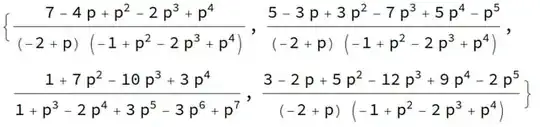

Note the 2nd term in that list (i.e. the answer starting from state $S_2$) is the answer I quoted for example 2 above.

Answer 2

[A partial answer illustrating the first method.]

State $1$ represents losing the game, so remove it from the system and condition the remaining transition probabilities on the event that the system does not transition from state $i$ to state $1$. In practical terms, this means that you delete from your transition matrix column $1$ and every row that had a $1$ in this column, and scale each remaining row $i$ by $1/(1-p_{1i})$. For your example system, this produces the reduced matrix $$P' = \begin{bmatrix}0&1&0&0&0 \\ 0&0&0&1&0 \\ q&0&0&0&p \\ 0&0&q&0&p \\ 0&0&0&0&1 \end{bmatrix}.$$ Applying standard techinques to this matrix, we can verify that the absorption probability is $1$ for any starting state and that the expected conditional absorption times are $$\begin{bmatrix}{3+q\over1-q^2} \\ {2+q+q^2\over1-q^2} \\ {1+3q\over1-q^2} \\ {1+q+2q^2\over1-q^2}\end{bmatrix}.$$