Also in the description of the
(finite-element-method)
tag it is said that
It is closely tied to the calculus of variations.
So let us consider the following variational integral:
$$
\iint \left[ \left(\frac{\partial \phi}{\partial x}\right)^2
+ \left(\frac{\partial \phi}{\partial y}\right)^2 \right] dx\,dy = \mbox{minimum}(\phi)
$$
In Finite Element methodology, as a rule, two coordinate systems are distinguished:
global coordinates $\,(x,y)$ - applicable to the whole domain of interest - and
local
coordinates $\,(\xi,\eta)$ - applicable to one element only. In this way a mapping is induced
between local and global coordinates. That mapping is called
isoparametric if every function
$\,f\,$ at an element - global coordinates being no exception - is expressed in the local coordinates, in the same way.
Thus we have $\,\phi(\xi,\eta)$ , $x(\xi,\eta)$ , $y(\xi,\eta)$ . And they all are similar expressions; examples following soon.
Of course we are mainly interested in the global derivatives $\,\partial \phi / \partial x\,$ and $\,\partial \phi / \partial y$ .
How can they be expressed in local coordinates? As follows.
Apply the chain rule for partial deriviatives, starting in the local coordinate system:
$$
\begin{cases} \large
\frac{\partial \phi}{\partial \xi} =
\frac{\partial \phi}{\partial x}\frac{\partial x}{\partial \xi} +
\frac{\partial \phi}{\partial y}\frac{\partial y}{\partial \xi} \\ \large
\frac{\partial \phi}{\partial \eta} =
\frac{\partial \phi}{\partial x}\frac{\partial x}{\partial \eta} +
\frac{\partial \phi}{\partial y}\frac{\partial y}{\partial \eta}
\end{cases}
$$
Two equations with two unknowns. They can be solved with Cramer's rule :
$$
\frac{\partial \phi}{\partial x} = \large
\frac{\frac{\partial \phi}{\partial \xi}\frac{\partial y}{\partial \eta} - \frac{\partial y}{\partial \xi}\frac{\partial \phi}{\partial \eta}}
{\frac{\partial x}{\partial \xi} \frac{\partial y}{\partial \eta} - \frac{\partial y}{\partial \xi}\frac{\partial x}{\partial \eta}}
$$ $$
\frac{\partial \phi}{\partial y} = \large
\frac{\frac{\partial x}{\partial \xi}\frac{\partial \phi}{\partial \eta} - \frac{\partial \phi}{\partial \xi}\frac{\partial x}{\partial \eta}}
{\frac{\partial x}{\partial \xi} \frac{\partial y}{\partial \eta} - \frac{\partial y}{\partial \xi}\frac{\partial x}{\partial \eta}}
$$
The simplest Finite Element in two dimensions is a
linear triangle :
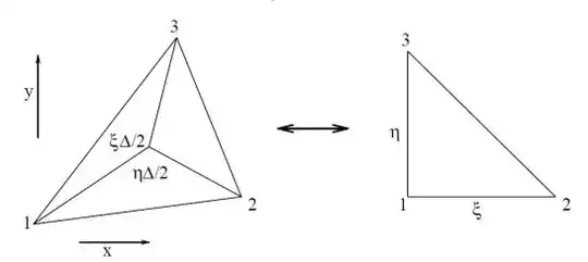
The vertex values of an arbitrary function $f$ at a linear triangle are interpolated by:
$$
f(\xi,\eta) = (1-\xi-\eta).f_1+\xi.f_2+\eta.f_3
$$
The very meaning of an isoparametric transformation is that we thus have:
$$
\begin{cases}
x(\xi,\eta) = (1-\xi-\eta).x_1+\xi.x_2+\eta.x_3 \\
y(\xi,\eta) = (1-\xi-\eta).y_1+\xi.y_2+\eta.y_3 \\
\phi(\xi,\eta) = (1-\xi-\eta).\phi_1+\xi.\phi_2+\eta.\phi_3
\end{cases}
$$
So there is no need to calculate the local derivatives separately. Just substitute for $\,f\,$ the "true" function, which is $\,x\,$ or $\,y\,$ or $\,\phi$ :
$$
\frac{\partial f}{\partial \xi} = f_2-f_1 \quad ; \quad \frac{\partial f}{\partial \eta} = f_3-f_1 \quad \mbox{with} \quad f = x,y,\phi
$$
Next take a look at Quadrilateral Interpolation :
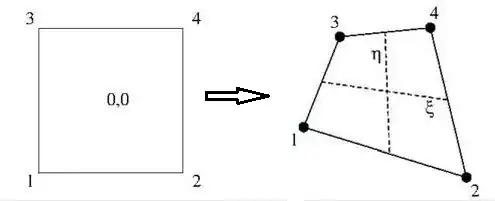
If the parent element of the quadrilateral on the left is $\left[-\frac{1}{2},+\frac{1}{2}\right]\times\left[-\frac{1}{2},+\frac{1}{2}\right]$ then we
have for an arbitrary function $f$ at the element on the right:
$$
f(\xi,\eta) = \left(\frac{1}{2}-\xi\right)\left(\frac{1}{2}-\eta\right)f_1
+ \left(\frac{1}{2}+\xi\right)\left(\frac{1}{2}-\eta\right)f_2 \\
+ \left(\frac{1}{2}-\xi\right)\left(\frac{1}{2}+\eta\right)f_3
+ \left(\frac{1}{2}+\xi\right)\left(\frac{1}{2}+\eta\right)f_4
$$
And for its derivatives, at vertex $(1)$ in particular:
$$
\frac{\partial f}{\partial \xi} = \left(\frac{1}{2}-\eta\right)(f_2-f_1)
+ \left(\frac{1}{2}+\eta\right)(f_4-f_3) \quad \Longrightarrow \quad
\frac{\partial f}{\partial \xi}(\eta = -1/2) = f_2-f_1\\
\frac{\partial f}{\partial \eta} = \left(\frac{1}{2}-\xi\right)(f_3-f_1)
+ \left(\frac{1}{2}+\xi\right)(f_4-f_2) \quad \Longrightarrow \quad
\frac{\partial f}{\partial \eta}(\xi = -1/2) = f_3-f_1
$$
Where again we must replace our dummy $\,f\,$ by the true functions $\,x,y,\phi\,$ in order to take care of the real thing.
It is readily observed now that all of the local derivatives at vertex $(1)$ of the quadrilateral are exactly the same
as all of the local derivatives at the linear triangle $(1,2,3)$. By symmetry, we can even conclude that the local derivatives
at any corner of the quadrilateral are exactly the same as the local derivatives at the triangle corresponding with
that corner. But then the same holds for the global derivatives $\,\partial \phi / \partial x\,$ and $\,\partial \phi / \partial y$ ,
because the analytical formula that expresses them into the local derivatives is the same for all (isoparametric) elements.
Last but not least, the analytical as well as the numerical formulation for the area elements does not make any difference too:
$$
dx\,dy = \frac{1}{4}\left[\frac{\partial x}{\partial \xi} \frac{\partial y}{\partial \eta} - \frac{\partial y}{\partial \xi}\frac{\partial x}{\partial \eta}\right]d\xi\,d\eta
$$
When specified for corner $(1)$, quadrilateral as well as triangle (each overlapping triangle counted half its weight/area):
$$
dx\,dy = \frac{1}{4}\left[(x_2-x_1)(y_3-y_1)-(y_2-y_1)(x_3-x_1)\right]d\xi\,d\eta
$$
Consequently, integration points at the vertices of a quadrilateral cannot be distinguished from
four overlapping triangles at the corners of that quadrilateral:
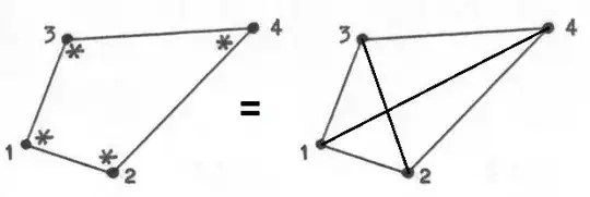
All mathematical components of both discretizations are the same in this variational integral:
$$
\iint \left[ \left(\frac{\partial \phi}{\partial x}\right)^2
+ \left(\frac{\partial \phi}{\partial y}\right)^2 \right] dx\,dy = \mbox{minimum}(\phi)
$$
So indeed: Finite Elements need not to be disjoint per se. Concerning the integration points:
Are there any two-dimensional quadrature that only uses the values at the vertices of triangles?


