Does a summation of two negative Gaussians with different standard deviations have a stationary point?

Question

I wanted to find the critical points of the (simple!) equation:

$$ B(w; \mu_1, \sigma_1, \mu_2, \sigma_2 ) = 1 - e^{ - \beta_1 (w - \mu_1)^2 } - e^{ - \beta_2 (w - \mu_2)^2}$$

Where $\beta_i = \frac{1}{2 \sigma^2_i}$ usually called the precision parameter of the Gaussian or RBF. Anyway, what I wanted in particular to solve is:

$$ B'(w; \mu_1, \sigma_1, \mu_2, \sigma_2 ) = - \beta_1 (w-\mu_1) e^{ - \beta_1 (w - \mu_1)^2 } - \beta_2(w - \mu_2)e^{ - \beta_2 (w - \mu_2)^2} = 0$$

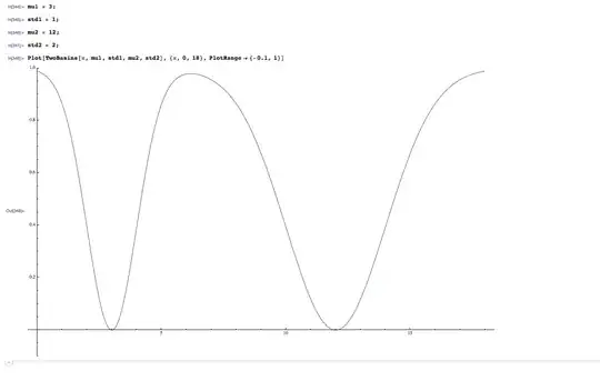
looking at the equation above I can't seem to find an easy way to make it zero. To make the first term zero we can choose $w = \mu_1 $ but that doesn't make the second term zero. Similarly, the other way round. However, it is super intuitively obvious that there are 2 minimums and 1 maximum since there are two dips defined by the upside down Gaussian (and in between them some maximum). I plotted this in mathematica to confirm that there must be these critical points and it seems I am correct:

however surprisingly I cannot find an easy way to express the critical points analytically. My initial goal is to at least have a way to express these 3 critical points for this 1 dimensional example if ever want to hope to find the critical points for higher dimensions.

Anyone knows how to do this?

---

My real intention is to be able to programmatically/systematically get the x-axis value between the two minimums that has exactly gradient equal to zero. Ideally able to generalize in higher dimensions.

For 1D and 2D I can sort of eye ball what the value should be by plotting things and then asking mathematics to tell me which value of $x$ leads to $\nabla f'(x) = 0$.

Answer 1

Let us make the change of variable $x = w - \frac{\mu_1+\mu_2}{2}$. Thus, using the identity $\beta_i = \exp\ln\beta_i$, the equation $B' = 0$ rewrites as $$ (x+\kappa) \exp\left(\ln\beta_1 -\beta_1 \left(x+\kappa\right)^2\right) + (x-\kappa) \exp\left(\ln\beta_2 -\beta_2 \left(x-\kappa\right)^2\right) = 0 \, , $$ where $\kappa = \frac{\mu_2 - \mu_1}{2}$. After dividing by $\exp Q_\kappa(x)$, where $$ 2 Q_\kappa(x) = \ln(\beta_1\beta_2) - \beta_1 \left(x+\kappa\right)^2 - \beta_2 \left(x-\kappa\right)^2 \, , $$ one obtains the identity $x \cosh P_\kappa(x) + \kappa \sinh P_\kappa(x) = 0$, where $$ 2 P_\kappa(x) = \ln(\beta_1/\beta_2) - \beta_1 \left(x+\kappa\right)^2 + \beta_2 \left(x-\kappa\right)^2 \, . $$ Therefore, $$ x + \kappa \tanh P_\kappa(x) = 0 \, . $$ Since $x\mapsto \kappa\tanh P_\kappa(x)$ is bounded and continuous, this equation has at least one solution.

• In the case $\kappa=0$, i.e. $\mu_1=\mu_2$, the only solution is $x=0$.

• In the case $\beta_1=\beta_2=\beta$, the equation rewrites as $$ 2\beta\kappa x = 2\beta\kappa^2 \tanh\left(2\beta\kappa x\right) . $$ The complete set of solutions is $$ x \in \left\lbrace \begin{aligned} & 0 \, ,\\ & {\pm \frac{u^*}{2\beta\kappa}} \quad\text{if}\quad 2\beta \kappa^2 > 1 \, , \\ \end{aligned} \right. $$ where $u^*>0$ satisfies $u^* = 2\beta\kappa^2\tanh(u^*)$. The value of $u^*$ can be computed numerically with Newton's method or any other suitable numerical method. To do so, an appropriate initial guess is required. For instance, one can use the value $u^* \approx \sqrt{3}\sqrt{2\beta\kappa^2 - 1}$, which is deduced from Taylor series. It seems hopeless to get an analytical expression of $u^*$.

• In the general case where $\mu_1\neq\mu_2$ and $\beta_1\neq\beta_2$, we introduce the polynomial factorization \begin{aligned} 2 P_\kappa(x) &= \left(\beta_2 - \beta_1\right) \left(x - x_0 - \Delta x\right) \left(x - x_0 + \Delta x\right) \\ &= \left(\beta_2 - \beta_1\right) \left( \left(x - x_0\right)^2 - {\Delta x}^2\right) , \end{aligned} $$ \text{where}\quad x_0 = \frac{\beta_1+\beta_2}{\beta_2-\beta_1}\kappa \quad\text{and}\quad \Delta x = \frac{\sqrt{4\beta_1\beta_2\kappa^2 - (\beta_2-\beta_1)\ln(\beta_1/\beta_2)}}{\beta_2-\beta_1}\, . $$ Maybe, a fine study would provide the exact number of solutions and their approximate location, but it seems hopeless to get an analytical expression of the solutions.

In order to find the abscissa of the local maximum, one can apply Newton's method and verify a posteriori that the returned value corresponds to a local maximum (the second derivative $B''$ must be negative). If $\beta_2/\beta_1\approx 1$, the initial guess $x=0$ can be used. Otherwise, if $\beta_2/\beta_1 \gg 1$ or $\beta_2/\beta_1 \ll 1$, the initial guess $x=\pm\kappa$ may be used.