There is a major flaw in the OP's (and many other people's) thinking.
Though it may be suggested by Classical Analysis all over the place, in Numerical Analysis the boundary conditions can not be considered as being separate from the differential equation(s).
Both the ODE/PDE and the BC are an integral part of the problem numerically. We shall illustrate by the most dramatic simplification possible:
$$
b(x) = f(x) = 0 \quad ; \quad a(x) = \pm v \quad \Longrightarrow \quad \frac{d\phi}{dx} = 0
$$
Where it is noticed that the information contained within $a(x) = \pm v$ has effectively disappeared.
Not so with the boundary conditions.
Let the integration domain be defined by $0 \le x \le L$, then there are two possible choices for the BC, say:
$$
\phi(0) = 1 \quad \mbox{xor} \quad \phi(L) = 1
$$
With $\phi(0) = 1$, the flow is in positive direction; with $\phi(L) = 1$, the flow is in negative direction.
And the upwind scheme must be adapted accordingly. Let the interval $0 \le x \le L$ be subdivided into
$N$ elements, then, with $k = 1,2,\cdots,N$ and $h = L/N$ :
$$
\frac{\phi_1-\phi_0}{h} = 0 \; , \;
\frac{\phi_2-\phi_1}{h} = 0 \; , \;
\cdots \; , \;
\frac{\phi_k-\phi_{k-1}}{h} = 0 \; , \;
\cdots \; , \;
\frac{\phi_N-\phi_{N-1}}{h} = 0
$$
$$ \begin{cases}
\phi_0 = 1 & \Longrightarrow & \phi_k := \phi_{k-1} & \mbox{starting with }\; k=1 \\
\phi_N = 1 & \Longrightarrow & \phi_{k-1} := \phi_k & \mbox{starting with }\; k=N \end{cases}
$$
With one and the same differential equation, there are two different numerical problems with two different schemes, finally.
Update. Q: "Is this right?" A: Yes and no. It depends entirely on the physical interpretation of the differential equation. The answer is yes if the ODE represents a convection / diffusion problem. But what if we augment it as follows:
$$
c(x)\phi(x)+a(x)\phi '(x)+b(x)\phi ''(x)=f(x)
$$
Then it can be an ODE for e.g. damped oscillations as well. And the latter is quite a different story numerically. Upwind differencing is a rather useless concept in that context (but I'm not an expert in the numerical treatment of wave equations). Similar arguments apply to the two-dimensional case. Additional reading:
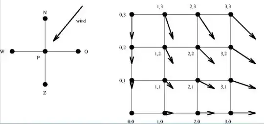
BONUS. As a second example, consider a 2-D case : pure convection of heat . The OP's unknown function $\phi$ is identified with $T$ (temperature) in concordance with this.
$$
a(x,y)\phi_x+b(x,y)\phi_{xx}+c(x,y)\phi_{y}+d(x,y)\phi_{yy}=f(x,y) \\
b(x,y)=d(x,y)=f(x,y)=0 \quad ; \quad a(x,y)=u(x,y) \quad ; \quad c(x,y) = v(x,y) \\
\Longrightarrow \quad u(x,y)\frac{\partial T}{\partial x} + v(x,y)\frac{\partial T}{\partial y} = 0
$$
Let the flow field be defined analytically by : $\;u(x,y) = x \; , \; v(x,y) = -y$ .
The discretization of the velocity field is:
$$
u = i \qquad ; \qquad v = - j
$$
The upwind scheme at a five point star is:
$$
U.(T_O-T_P) + V.(T_N-T_P) = 0
$$
In our case - look at the wind - it is seen that $U = u$ and $V = -v$ .
Working out the upwind scheme for the temperatures therefore results in:
$$
(i+j).T_{i,j} = i.T_{i-1,j} + j.T_{i,j+1}
$$
Assume a linear temperature profile on top, where the fluid comes in: $T_{i,3} = i$. The walls are always streamlines, hence $T_{0,j} = T_{i,0} = 0$. Now the temperatures in the rest of the field can be calculated by hand, for example:
$$
(1+2).T_{1,2} = 1.0 + 2.1 = 2 \quad \Longrightarrow \quad T_{1,2} = 2/3
$$
After six of these simple calculations the temperature field reads as follows:
        0     1     2     3
        0    2/3   4/3    2
        0    1/3   2/3    1
        0     0     0     0
Take a look at the temperature profile at the outflow opening: it is exactly as expected!
Even better. It can be proved that the discrete temperature field for an $N\times N$ grid
is given in general by: $T_{i,j} = i.j/N$ . Which corresponds
exactly with the analytic solution: $T(x,y) = x.y$ .
Who has said that upwind schemes are somehow "less accurate"?
OK, and now
reverse all velocities (change signs). This will
not change the differential equation, but the inflow opening shall be at the former outflow opening. And the upwind scheme must be adapted accordingly.
