As Ron Maimon has said in the comments, the IQ scale is defined so that it gives a normal distribution with a mean of $100$ and a standard deviation of $15$. This is possible for any test score with a continuous distribution $f$. If the subject's score on the test is $s$, their IQ will be given by:
$$\text{IQ}=100+15\sqrt 2\;\text{erfc}^{-1}\left(2-2\int_{-\infty}^sf(x)dx\right)$$
To see that this gives a normal distribution, invert the equation above:
$$\int_{-\infty}^sf(x)dx = 1 - \frac{1}{2}\;\text{erfc}\left(\frac{\text{IQ} - 100}{15\sqrt 2}\right)$$
The left-hand side is the cumulative distribution function (CDF) of the test scores and the right-hand side is the expression for the CDF of a normal distribution.
It may sound weird to define IQ so that it fits an arbitrary distribution, but that's because IQ is not what most people think it is. It's not a measurement of intelligence, it's just an indication of how someone's intelligence ranks among a group:
The I.Q. is essentially a rank; there are no true "units" of intellectual ability.
[Mussen, Paul Henry (1973). Psychology: An Introduction. Lexington (MA): Heath. p. 363. ISBN 978-0-669-61382-7.]
In the jargon of psychological measurement theory, IQ is an ordinal scale, where we are simply rank-ordering people. (...) It is not even appropriate to claim that the 10-point difference between IQ scores of 110 and 100 is the same as the 10-point difference between IQs of 160 and 150.
[Mackintosh, N. J. (1998). IQ and Human Intelligence. Oxford: Oxford University Press. pp. 30–31. ISBN 978-0-19-852367-3.]
When we come to quantities like IQ or g, as we are presently able to measure them, we shall see later that we have an even lower level of measurement—an ordinal level. This means that the numbers we assign to individuals can only be used to rank them—the number tells us where the individual comes in the rank order and nothing else.
[Bartholomew, David J. (2004). Measuring Intelligence: Facts and Fallacies. Cambridge: Cambridge University Press. p. 50. ISBN 978-0-521-54478-8.]
From those quotes, you can deduce that any other information about the original distribution of scores in the actual test used to measure intelligence, like skewness and kurtosis, is simply lost.
The reason for choosing a Gaussian, and with those parameters, is mostly historical. But it's also very convenient. It turns out that you'd need about as many people as have ever existed to get someone to be ranked as an IQ of zero and someone else to be ranked as $200$ (roughly $1$ in $76$ billion). So in practice, IQ is limited to the interval $[0, 200]$ (no, there's no such thing as $300$ IQ. Sorry Sidis). Also, the dumbest person alive would have an IQ of $5$ and the smartest person $195$ ($1$ in $8.3$ billion). If you could theoretically apply the same test to trillions of people, then you'd get IQs above $200$ and even negative IQs. Obviously, the results will be different for different tests, and you might question whether any of the tests have really anything to do with actual intelligence.
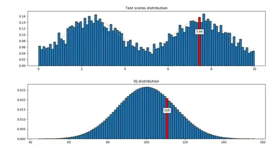
To illustrate how you'd calculate IQ in practice, I made a Python script which takes an arbitrary distribution of scores in a test, generates a sample of $10$ thousand results and uses that to calculate the IQ of an additional participant based on their score in the same test. The plot shows the distribution of scores and how it's transformed into a normal distribution when converted to IQ. The score and IQ of the new participant are shown in red.
import bisect
import numpy as np
from scipy.special import erfcinv
from scipy.stats import rv_continuous
N_SAMPLES = 10000
np.random.seed(0)
Start with any continuous distribution for the test scores.
In this case, it's a multimodal distribution.
def scores_pdf(x):
    return (2-np.cos(2np.pix/5))/20
class dist_gen(rv_continuous):
    def _pdf(self, x):
        return scores_pdf(x)
We restrict the score to be between zero and ten.
dist = dist_gen(a=0, b=10)
scores = dist.rvs(size=N_SAMPLES)
scores = list(sorted(scores))
Convert from percentile to IQ
def p_to_iq(p):
    return 100 + 15np.sqrt(2)erfcinv(2 - 2*p)
The scores are not even used yet, only their ordering.
iqs = [p_to_iq(k/N_SAMPLES) for k in range(1, N_SAMPLES)]
Calculating the percentile for a finite sample set depends on
how it is defined. This function returns the smallest and the
highest values.
def get_percentile_bounds(score):
    size = len(scores)
    # Number of samples lower than 'score'
    lower = bisect.bisect_left(scores, score)
    # Number of samples greater than 'score'
    greater = size - bisect.bisect_right(scores, score)
    return lower/(size+1), (size-greater+1)/(size+1)
We use only the definition of percentile closest to the average.
(This is arbitrary and irrelevant for large sample sets)
def get_iq(score):
    p1, p2 = get_percentile_bounds(score)
    if abs(p1-0.5) < abs(p2-0.5):
        return p_to_iq(p1)
    return p_to_iq(p2)
A new subject performs the test.
new_score = dist.rvs()
new_iq = get_iq(new_score)
print(new_score, new_iq)
import matplotlib.pyplot as plt
from scipy.stats import norm as gaussian
N_BINS = 100
def highlight_patch(value, patches, axis, fmt):
    left, bottom = patches[0].get_xy()
    width = patches[0].get_width()
n = int((value - left)//width)
patches[n].set_fc('r')

x = left + (n+0.5)*width
y = bottom + 0.7*patches[n].get_height()
axis.text(x, y, fmt%(value),
          horizontalalignment='center',
          verticalalignment='center',
          bbox=dict(facecolor='white',alpha=0.9))


fig, axes = plt.subplots(nrows=2, ncols=1)
n, bins, patches = axes[0].hist(
    scores,
    bins=100,
    density=True,
    edgecolor='black')
highlight_patch(new_score, patches, axes[0], '%.2f')
x = np.linspace(scores[0], scores[-1], num=200)
axes[0].plot(x, [scores_pdf(k) for k in x], ':')
axes[0].set_title('Test scores distribution')
n, bins, patches = axes[1].hist(
    iqs,
    bins=100,
    density=True,
    edgecolor='black')
highlight_patch(new_iq, patches, axes[1], '%.0f')
x = np.linspace(iqs[0], iqs[-1], num=200)
axes[1].plot(x, [gaussian.pdf(k, 100, 15) for k in x], ':')
axes[1].set_title('IQ distribution')
fig.tight_layout()
plt.show()