10

I've inherited some numerical analysis code that integrates a 2D function that is only known at a large set of unstructured points.

The way it does this is by Delauney triangulating the domain using the sample points, and then calculating the area of the Voronoi cell at each point, and using that as the weight associated with each point. Neglecting edge effects the sum of the areas will total up to the area of the domain, and so it seems a valid approach - but not how I'd approach it.

I'd use the Delauney triangulation and derive the weights from the finite element style basis function at each vertex. (1/3 the area of the sum of the triangles with the same vertex.). Again the functions weights sum to the area of the domain.

It seems in 1D the two approaches would be the same, but I don't think this is the case for 2D.

So my question is are there known advantages/disadvantages for each style of numerical integration?

  • I can't think of a direct answer to this, but I have a comment to make. The approaches are conceptually similar: find an interpolant of the function, then integrate the interpolating function. One interpolant is piecewise constant on Voronoi cells, one is piecewise linear on Delaunay triangles (or something like this, I can't quite tell if this is what you mean). Of course you could choose other interpolation schemes too. Linear interpolation could be more accurate, depending on the properties of the function. – Kirill Sep 13 '14 at 23:20
  • 1
    If you don't get a good answer here, you might consider asking on http://scicomp.stackexchange.com/. –  Sep 14 '14 at 10:36
  • One trivial observation: the Voronoi method is continuous in the sample locations, while the Delaunay method can change discontinuously if the samples are perturbed. –  Sep 14 '14 at 10:41
  • Since the Voronoi is the geometric dual of the Delaunay diagram they have the same level of geometric dependence on the sample locations (i.e. the underlying mesh geometry is identical). However the Voronoi based approximation is constant on the cells, while the Delaunay approximation is linear on each triangle - meaning that the Delaunay approximation has better continuity in sample location. Perturbing a sample location must actually change the underlying mesh topology to generate a discontinuity for Delaunay, while in Voronoi the slight non-topological changes move cell discontinuities). – Michael Anderson Sep 15 '14 at 00:43
  • If you put "@Rahul" somewhere in your comment I get notified of your reply. It doesn't matter whether the auxiliary function you've constructed is continuous or not. The final integral you compute is ultimately a linear combination of (a) the areas of the Voronoi regions, or (b) the total area of the adjacent triangles of each sample point. With Voronoi, the areas of the Voronoi regions always change continuously if you move the sample points. But with Delaunay, the mesh topology can change, and in that case the result of the integral will change discontinuously upon moving a point. –  Sep 16 '14 at 06:53
  • @Rahul - ah that's the key point that I missed in your comment/answer - While the topology of the Voronoi diagram will change disontinouosly (as the Delaunay triangulation changes), the areas of the Voronoi cells only change continuously and locally - in contrast the areas of the Delaunay triangulations will change dicontinuously and non-locally. If you put it as an answer I'll accept it. – Michael Anderson Sep 16 '14 at 08:29
  • @MichaelAnderson: There is a definite (and continuous) ratio between Delaunay style and Voronoi style areas - see my answer below. Therefore I cannot comprehend this argumentation. – Han de Bruijn Sep 18 '14 at 09:09
  • @HandeBruijn You can see the relevant issue clearly in this wikipedia image http://en.wikipedia.org/wiki/Delaunay_triangulation#mediaviewer/File:Delaunay_triangulation_does_not_minimize_edge_length.gif Consider the weight associated with the left vertex as the central vertices move. The Delaunay weight is discontinuous, while the Voronoi one is not. – Michael Anderson Sep 19 '14 at 02:23
  • I appreciate the effort everyone has put into this question - there's still no clear answer, but I think @Rahul has given me some insight into some cases where Voronoi might be preferable - so rather than let the bounty go to waste I'm awarding it to him. – Michael Anderson Sep 19 '14 at 02:38
  • @HandeBruijn I think you may be close to having a proper comparison based on some of your ideas, but I don't think it's solid yet - and I'm not sure how to take it the extra steps. – Michael Anderson Sep 19 '14 at 02:40
  • @MichaelAnderson: Please also read my latest comments on Rahul's answer. To be honest, I still feel a bit uncomfortable with the whole problem. Wish I could think of a shortcut that simply avoids triangulation / Voronoi tessellation in the first place. – Han de Bruijn Sep 19 '14 at 12:40
  • @MichaelAnderson: One last remark concerns the boundaries: The chain is as strong as the weakest link. With the Delaunay triangulation, the boundaries are convex, an artefact of the method. With the Voronoi tesselation, the situation is even worse: the cells at the boundary are extending to infinity. – Han de Bruijn Sep 19 '14 at 19:32
  • As suggested by @Rahul a version of this has been posted on scicomp.SE : http://scicomp.stackexchange.com/questions/14802/comparison-between-voronoi-and-delaunay-2d-quadrature-methods – Michael Anderson Oct 08 '14 at 03:12
  • Work on the subject continued in november-december 2021: Voronoi & Delaunay and What is the proper way to do DTFE . – Han de Bruijn Jan 01 '22 at 10:35

3 Answers3

4

Apart from the observation that the two methods seem to be (or rather should be) equivalent, using the Delaunay triangulation, without the Voronoi detour, seems to be the most straightforward.
Furthermore it is more convenient to first determine the integral over one (Delaunay) triangle and then simply sum up over all triangles; nothing is gained with gathering triangles at the same vertex, for the reason that a summation of numbers can be in any order.
Precise formulation for one triangle $\Delta$ with vertices $(x_1,y_1),(x_2,y_2),(x_3,y_3)$ and function values $(f_1,f_2,f_3)$ at these vertices (in case you didn't know this already): $$ \iint_{\Delta} f(x,y)\,dx\,dy = \frac{1}{2} \det\begin{bmatrix} (x_2-x_1) & (x_3-x_1) \\ (y_2-y_1) & (y_3-y_1) \end{bmatrix} \frac{f_1+f_2+f_3}{3} $$ Then sum up over all triangles in the domain / mesh $\Omega$ : $$ \iint_{\Omega} f(x,y)\,dx\,dy = \sum_{\Delta} \iint_{\Delta} f(x,y)\,dx\,dy $$ And that's it. So I'd vote for your approach, apart from minor details.

Sideways note. Actually, Delaunay triangles and Voronoi regions are dual to each other.
The former concept is the more favorite with Finite Element Methods, while the latter concept is the more favorite with Finite Difference/Volume methods. My personal bias is the unification of both; Voronoi regions are at page 13 in the following reference : 2-D Elementary Substructures .

Delaunay and Voronoi regions.
enter image description here

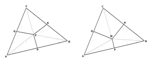
  • Picture on the left: (Delaunay) triangle with medians and regions tentatively called Delaunay regions (hoping this nomenclature has not been claimed already somewhere)
  • Picture on the right: same triangle with perpendicular bisectors and Voronoi regions
It is easy to show that the area of a Delaunay region is $1/3 \times$ the area of the (Delaunay) triangle.
Proof. Without loss of generality, let $A = (0,0)$ , $B = (x_B,y_B)$ , $C = (x_C,y_C)$ , then the area of e.g. the Delaunay region $APZQ$ is: $$ \frac{1}{2} \det\begin{bmatrix} x_B/2 & (x_B+x_C)/3 \\ y_B/2 & (y_B+y_C)/3 \end{bmatrix} + \frac{1}{2} \det\begin{bmatrix} (x_B+x_C)/3 & x_C/2 \\ (y_B+y_C)/3 & y_C/2 \end{bmatrix} = \frac{1}{3} \times \frac{1}{2} \det\begin{bmatrix} x_B & x_C \\ y_B & y_C \end{bmatrix} $$ So we may safely conclude that the numerical integration procedure as proposed in this answer is equivalent with numerical integration over Delaunay regions (collected around a vertex).
Finding the area of a Voronoi region is far more complicated (I think). It is clear from the pictures, however, that weighting function values with Delaunay regions is at least different from weighting function values with Voronoi regions (except for equilateral triangles).

UPDATE. Without loss of generality again, let $A = (0,0)$ , $B = (x_B,y_B)$ , $C = (x_C,y_C)$ , then the area of e.g. the Voronoi region $APMQ$ is: $$ V = \frac{\left[(x_B^2+y_B^2) - (x_B x_C + y_B y_C)\right]\left[x_C^2+y_C^2\right]} {8(x_B y_C- y_B x_C)} + \frac{\left[(x_C^2+y_C^2) - (x_B x_C + y_B y_C)\right]\left[x_B^2+y_B^2\right]} {8(x_B y_C- y_B x_C)} $$ Coded in a little (Delphi) Pascal program - the function call $V(A,B,C)$ is to be memorized:

program Voronoi;
type point = record x,y : double; end;
function V(A,B,C : point) : double; { Area of Voronoi Region in Delaunay triangle } var O1,O2 : double; p,q : point; begin p.x := B.x-A.x; p.y := B.y-A.y; q.x := C.x-A.x; q.y := C.y-A.y; O1 := (-q.yp.y+p.xp.x+p.yp.y-p.xq.x)(q.xq.x+q.yq.y) / (p.xq.y-p.yq.x)/8; O2 := (-q.yp.y+q.xq.x+q.yq.y-p.xq.x)(p.xp.x+p.yp.y) / (p.xq.y-p.yq.x)/8; V := O1+O2; end;
procedure test; { Sum of Voronoi areas must be Area of Delaunay triangle } var A,B,C,p,q : point; begin Random; Random; p.x := Random; p.y := Random; q.x := Random; q.y := Random; A.x := 0; A.y := 0; B.x := p.x; B.y := p.y; C.x := q.x; C.y := q.y; Writeln(V(A,B,C) + V(B,C,A) + V(C,A,B), ' =',(p.xq.y-p.yq.x)/2); end;
begin test; end.
Thus, quite in general, the numerical integration procedure is as follows: $$ \iint_{\Delta} f(x,y)\,dx\,dy = w_1 f_1 + w_2 f_2 + w_3 f_3 \qquad ; \qquad \iint_{\Omega} f(x,y)\,dx\,dy = \sum_{\Delta} \iint_{\Delta} f(x,y)\,dx\,dy $$ Where:

  • $w_1=w_2=w_3=1/3 \times$ area of triangle , for the Delaunay regions approach
  • $w_1 = V(A,B,C)\, , w_2 = V(B,C,A)\, , w_3 = V(C,A,B)$ , for the Voronoi regions approach
Consider all Delaunay / Voronoi regions around a vertex. For simplicity, assume that the associated triangles form a regular polygon with $N$ edges, such that each top angle of a triangle is $\phi=2\pi/N$ . All triangles are isoceles, hence $\;x_B^2+y_B^2=x_C^2+y_C^2=L^2\;$ and we can easily determine the ratio ( area of a Delaunay region ) / ( area of Voronoi region ) , with the cosine rule for an inner product and the sine rule for a determinant: $$ \frac{L^2\sin(\phi)/2/3}{2\left[L^2-L^2\cos(\phi)\right]L^2/\left[8L^2\sin(\phi)\right]} = \frac{2}{3}\frac{\sin^2(\phi)}{1-\cos(\phi)} \quad \Longrightarrow \\ \frac{\mbox{Delaunay}}{\mbox{Voronoi}} = \frac{2}{3}\left[\,1+\cos(\phi)\,\right] $$ It follows that Delaunay = Voronoi for $\,1+\cos(\phi) = 3/2\,$ hence $\,\phi=\pi/3$ , as expected (equilateral triangles) . Furthermore Delaunay > Voronoi for $\,\phi<\pi/3\,$ and Voronoi > Delaunay for $\,\phi>\pi/3$ . Especially for obtuse triangles (negative cosine) the ratio can become nearly zero, which means that the Voronoi regions can become much larger than the Delaunay regions, thereby giving a seemingly unreasonable high weight to an associated function value.
Let $\;a=\sqrt{x_B^2+y_B^2}\;$ and $\;b=\sqrt{x_C^2+y_C^2}\;$ . Then for those who want the above WLOG : $$ \frac{\mbox{Delaunay}}{\mbox{Voronoi}} = \frac{4/3\,a^2b^2\left[1-\cos^2(\phi)\right]}{2a^2b^2-ab(a^2+b^2)\cos(\phi)} $$ Solving for the three cases $\;<1,=1,>1\;$ is then equivalent with solving a quadratic equation for $<0,=0,>0$ , i.e. where the following parabola is positive/zero/negative, with $\;x=\cos(\phi)$ : $$ y = x^2-\frac{3}{4}\frac{a^2+b^2}{ab}x+\frac{1}{2} $$
Han de Bruijn
  • 17,070
  • Can you elaborate on why you feel the two should be equivalent. Naively I might expect the Delaunay to have a better order of convergence than Voronoi, since it is based on linear interpolation. (I'm not sure that this is the case though.) – Michael Anderson Sep 15 '14 at 00:45
  • As is clear from the updated answer, I've withdrawn my claim that Delaunay and Voronoi are equivalent. Since both methods finally result in just weights for the function values, I don't see what linear or not has to do with a better order of convergence. – Han de Bruijn Sep 18 '14 at 09:14
  • 2
    Simpsons method and the trapezoidal method are also just nodal weights for calculating a 1-D integral. Yet they have different orders of convergence for smooth functions. Correctly choosing the weights has everything to do with rates of convergence. – Michael Anderson Sep 19 '14 at 02:35
4

The PhD thesis of Willem Schaap ("DTFE: the Delaunay Tessellation Field Estimator" University of Groningen, Kapteyn Astronomical Institute) discusses Voronoi versus Delaunay weighting schemes for re-sampling irregular point sets on to a regular grid: http://irs.ub.rug.nl/ppn/298831376.

Once re-sampled you can integrate, take FFT's and so on. Schaap gives cogent reasons as to why the Delaunay weighting (DTFE) is to be preferred over Voronoi weighting (VTFE). This has been used widely in the analysis of astronomical data sets. There are generalisations to get higher levels of continuity, if necessary, using "Natural Neighbours" on a Delaunay tessellation (http://arxiv.org/abs/1107.1488).

  • Its a very interesting thesis, but it seems to be more related estimating density functions using a combination of Voronoi and Delaunay based methods. While there are certainly similarities between density estimation and numerical integration, the thesis does not seem to directly address this. (Other than from the aspect of global mass conservation, which both the Delaunay and Voronoi methods outlined in the original question both achieve) – Michael Anderson Oct 14 '14 at 01:46
  • Indeed true. But once one has an optimal density on a grid, standard (well understood, straightforward code) methods of filtering, integration, evolution and so on take over. In practical terms this is a great advantage until the number of points gets into the billions. In my field (cosmology) there is little reason to stick with the original point distribution unless, perhaps, one is interested in (multi)fractal dimensions. – JonesTheCosmologist Oct 14 '14 at 23:30
  • Obviously I'm missing something but I cant see how to get from an approximation of the density of a point process to the integral of values at the points. – Michael Anderson Oct 15 '14 at 00:12
  • The re-sampling onto a grid is, in effect, a reconstruction of the function that underlies the values at the sampled points. It's little different from Lagrangian Interpolation in one dimension. It can be shown that, given certain mathematical conditions, the integral of the data given on the point set converges to the integral of the underlying function in the limit of a large sample of points or a large volume. I should add that this re-sampling is only of benefit in 2-D and 3-D as per the original question. In higher dimensions this is hopelessly inefficient (use MCMC). – JonesTheCosmologist Oct 16 '14 at 09:51
3

Another not complete answer, but I've actually performed some numerical studies of the two cases: TLDR; For most cases they're almost indistinguishable.

I suspect that this is related to the observations in Han de Bruijn's answer - and that the Delaunay and Voronoi regions are close to the same size, since the Delaunay triangulation tries to produce "nice" triangles.

All my studies were in the $[-1,1]\times[-1,1]$ square, using between 100 and 10,000 points and the results taken from 20 repeats.

The points were stratified (as they are in my real data), such that the points are essentially grid points + uniform noise equal to the grid spacing. (This results in better convergance and nicer triangulations than would be expected from truly random data). The edges of the domain were handled by adding "ghost" points which contributed to the triangulation and calculated weight of neighbouring non-ghost points, but were not used in the summation to calculate the integrals.

The functions I used were:

X

$$f(x,y) = x$$

Constant Ball

$$f(x,y) = \begin{cases} 1 & r < 0.75 \\ 0 & \textrm{otherwise} \end{cases}$$

Ball X

$$f(x,y) = \begin{cases} x & r < 0.75 \\ 0 & \textrm{otherwise} \end{cases}$$

Ball XY

$$f(x,y) = \begin{cases} x\;y & r < 0.75 \\ 0 & \textrm{otherwise} \end{cases}$$

Smooth Ball XY

$$f(x,y) = \begin{cases} w(r)\;x\;y & r < r_{max} \\ 0 & \textrm{otherwise} \end{cases}$$

Where

$$ r_{max}=0.85 \\ z = r/r_{max} \\ w(r) = (1-z)^2 * (2z+1) $$

Graphs of the convergence can be seen here (mean absolute error are the left graphs, max absolute error from the 20 iterations is the right graph). Convergence For Different methods
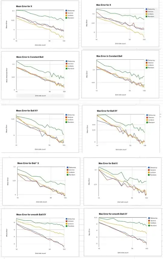
, Blue lines are Delaunay, Red Voronoi, Yellow has all weights set to 1.0, and Green has them set to random 0-1 values.

The interesting results are, the Blue and Red lines seem qualitatively the same in all cases. They only differ from the Yellow lines for two cases:

  1. $f(x,y)=x$ for which Voronoi and Delaunay are behaving worse than Uniform case - suggesting they're not behaving correctly at the edges on the domain. However this appears to be a constant offset in log-log space, suggesting that it is not a degredation in the rate of convergence.

  2. The smooth ball - where they both behave better than uniform, and this appears to be a difference in the rate of convergence - suggesting that the convergence is limited by the discontinuity across the ball edges in the other cases.

The best that I can conclude from this is that for several simple cases the two algortithms have similar convergance rates, in some cases better than uniform weighting, but you need to be careful about edge effects.

It may be interesting to examine A smooth X Ball case - but I've run out of time to burn on this.

  • +1 Can you find the slope of the lines in log-log space? That would indicate the order of convergence. –  Sep 17 '14 at 19:11
  • The slopes are, for the smooth ball case: -3.14, -3.00, -1.95, -0.91. (I tried to give public access to the raw data, but google spreadsheets wasn't playing nice.) – Michael Anderson Sep 18 '14 at 08:56