A nice way to think about it is to notice that a function from any finite set to itself can be represented as a tuple, with the $i$th element giving the image of $i$ under the function: for example, $(2,3,4,1)$ is a representation of a function from the set $\{1,2,3,4\}$ to itself.
I'll write all my code using MATLAB syntax, as I think it's particularly easy to read, and arrays index from 1, which is sometimes pleasant for mathematicians.
Function composition is composition of tuples, and it can be computed in linear time:
function h = compose(f,g)
    disp('Called compose')
    for i = 1:length(f)
        h(i) = f(g(i));
    end
end
I've inserted a line to display a message every time the function composition routine is called. The squaring operator is then easily defined:
function f2 = square(f)
    f2 = compose(f,f);
end
And finally our exponentiation routine is:
function h = exponentiate(f,n)
    if n == 1                     % The base case
        h = f;
    elseif mod(n,2) == 0
        g = exponentiate(f,n/2);
        h = square(g);
    else
        g = exponentiate(f,(n-1)/2);
        h = compose(f,square(g));
    end
end
We can now define a function and exponentiate it:
>> f = [2,3,4,5,1];

>> exponentiate(f,2)

Called compose

ans =

     3     4     5     1     2

>> exponentiate(f,16)

Called compose
Called compose
Called compose
Called compose

ans =

     2     3     4     5     1

>> exponentiate(f,63)

Called compose
Called compose
Called compose
Called compose
Called compose
Called compose
Called compose
Called compose
Called compose
Called compose

ans =

     4     5     1     2     3
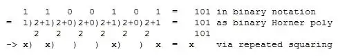
And there you have it - the composition function is called approximately $\log_2(x)$ times when we compose the function with itself $x$ times. It takes $O(n)$ time to do the function composition and $O(\log x)$ calls to the composition routine, for a total time complexity of $O(n\log x)$.