Probability: the average times to make all the balls the same color

Question

Suppose there are n balls with different colors with each other in a bag. In one loop, One take two balls in sequence out of the bag and replace them with two balls with the same color of the first ball. Q: how many loops does it take to make all the balls the same color on average?

Answer 1

Very interesting problem, and this is rather an write-up of a computation experiment to explore it.

As it has been already pointed out in the comments, the dynamics of the urn can be described by a Markov chain on integer partitions of $n$. Let $\{m_1, \ldots, m_k \}$ be such a partition. Suppose $i$, $j$, such that $1 \leqslant i,j\leqslant k$, are the two types of ball drawn in a loop. If $i=j$, the urn remains in the same state with the probability $\frac{m_i}{n} \frac{m_i-1}{n-1}$, otherwise it transitions to a new partition with $m_i$ increased by one, and $m_j$ decreased by 1 with probability $\frac{m_i}{n} \frac{m_j}{n-1}$.

Here a Mathematica code that constructs such a finite Markov process:

computeProbabilities[p : {n_}, as_] := {{as[p], as[p]} -> 1}
computeProbabilities[p_List, as_] := 
Module[{n = Length[p], tot = Total[p], bag, pnew},
  bag = {};
  Do[
   If[i == j,
    If[p[[i]] > 1, 
       AppendTo[bag, {as[p], as[p]} -> p[[i]]/tot (p[[i]]-1)/(tot-1)]
    ],
    pnew = DeleteCases[p + UnitVector[n, i] - UnitVector[n, j], 0]; 
    pnew = Sort[pnew, Greater];
    AppendTo[bag, {as[p], as[pnew]} -> p[[i]] p[[j]]/tot/(tot - 1)]
   ], {i, n}, {j, n}];
  Normal[Total /@ GroupBy[bag, First -> Last]]
]

buildMarkovProcess[n_Integer?Positive] := Module[{ip, as, tm, lip},
  ip = IntegerPartitions[n]; 
  as = AssociationThread[ip, Range[lip = Length[ip]]];
  tm = SparseArray[Flatten[computeProbabilities[#, as] & /@ ip], {lip, lip}];
  DiscreteMarkovProcess[lip, tm]
]

The least number of loops needed to get all ball to have the same color is the first passage time distribution to reach partition $\{n\}$, which has index 1 in this code, and which is the absorbing state of the Markov chain.

StepsToSameColorDistribution[n_Integer?Positive] := 
 FirstPassageTimeDistribution[buildMarkovProcess[n], 1]

We can now ask for the mean number steps $K_n$ needed to reach the absorbing state:

In[392]:= Table[{n, Mean[StepsToSameColorDistribution[n]]}, {n, 2, 12}]

Out[392]= {{2, 1}, {3, 4}, {4, 9}, {5, 16}, {6, 25}, {7, 36}, {8, 
  49}, {9, 64}, {10, 81}, {11, 100}, {12, 121}}    

Which conforms to the pattern $\mathbb{E}(K_n) = (n-1)^2$:

In[392]:= FindSequenceFunction[%, n]

Out[392]= (-1 + n)^2

The intriguing feature of the $K_n$ random variable is revealed by looking at its probability generating function:

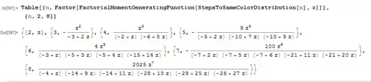
This reveals that $K_n - (n-1)$ can be represented as a sum of $n-2$ independent geometric random variables with some specific distinct failure probabilities. Putting this into code:

toTransformedDistribution[n_Integer] := Module[{pgf, den, z, ps, fgm, xvec},
  fgm = FactorialMomentGeneratingFunction[StepsToSameColorDistribution[n], z];
  pgf = Factor[fgm];
  den = Denominator[pgf];
  If[FreeQ[den, z],
   TransformedDistribution[n - 1, Distributed[x, GeometricDistribution[1/2]]]
   ,
   ps = Part[Rest[FactorList[den]], All, 1];
   ps = Map[1 + Coefficient[#, z, 1]/Coefficient[#, z, 0] &, ps];
   xvec = Array[x, n - 2];
   TransformedDistribution[n - 1 + Total[xvec], 
      Distributed[xvec, ProductDistribution @@ Map[GeometricDistribution, ps]]]
  ]
]

We check consistency:

In[424]:= 
Table[FactorialMomentGeneratingFunction[toTransformedDistribution[n], 
    z] == FactorialMomentGeneratingFunction[
    StepsToSameColorDistribution[n], z], {n, 2, 8}] // Simplify

Out[424]= {True, True, True, True, True, True, True}

And now show the decomposition. $K_3 \stackrel{d}{=} 2 + X_1$, where $X_1 \sim \mathrm{Geo}\left(\frac{1}{3}\right)$:

In[431]:= toTransformedDistribution[3]

Out[431]= TransformedDistribution[
 2 + X1, Distributed[X1, GeometricDistribution[1/3]]

$K_4 \stackrel{d}{=} 3 + X_1 + X_2$, where $X_1 \sim \mathrm{Geo}\left(\frac{1}{2}\right)$ and $X_2 \sim \mathrm{Geo}\left(\frac{1}{6}\right)$, and $X_1$ and $X_2$ are independent:

In[432]:= toTransformedDistribution[4]

Out[432]= TransformedDistribution[
 3 + X1 + X2, {X1, X2} \[Distributed] 
  ProductDistribution[GeometricDistribution[1/2], 
   GeometricDistribution[1/6]]]

Likewise $K_5 = 4 + X_1 + X_2 + X_3$, where $X_1 \sim \mathrm{Geo}\left(\frac{3}{5}\right)$, $X_2 \sim \mathrm{Geo}\left(\frac{3}{10}\right)$, $X_3 \sim \mathrm{Geo}\left(\frac{1}{10}\right)$, and $X_1$, $X_2$ and $X_3$ are independent:

In[433]:= toTransformedDistribution[5]

Out[433]= TransformedDistribution[
 4 + X1 + X2 + X3, {X1, X2, X3} \[Distributed] 
  ProductDistribution[GeometricDistribution[3/5], 
   GeometricDistribution[3/10], GeometricDistribution[1/10]]]

Of course, if anyone can offer an insight into why such a decomposition should take place, I would tip my hat to the tune of a bonus.

---

Added: Further experimental math analysis reveals a pattern to the geometric distribution failure rates in the decomposition of $K_n$, specifically $$ K_n \stackrel{\mathrm{law}}{=} n - 1 + \sum_{i=1}^{n-2} X_i, \quad X_m \sim \mathrm{Geom}\left(\frac{m (m+1)}{n(n-1)}\right) \, \mathrm{ for } \,\, 1 \leqslant m \leqslant n-2 $$ Hence, denoting $p_i = i(i+1)/n/(n-1)$ $$\begin{eqnarray} \mathbb{E}\left(K_n\right) &=& n-1 + \sum_{i=1}^{n-2} \left(\frac{1-p_i}{p_i}\right) = n - 1 + \sum_{i=1}^{n-2} \left( \frac{n(n-1)}{i} - \frac{n(n-1)}{i+1} - 1 \right) \\ &\stackrel{\mathrm{telesc.}}{=}& (n-1) + \frac{n(n-1)}{1} - \frac{n(n-1)}{n-1} - (n-2) = 1 + n(n-1) - n \\ &=& \fbox{$\left(n-1\right)^2$} \end{eqnarray} $$

The question remains open as to why $K_n$ can be decomposed into this sum of independent geometric random variables?