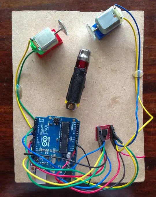
Finally I had time to do some coding and I can generate your images on computer. The mathematics is fairly simple. The backbone of the simulation are two functions
- Ray & plane intersection: Let's have ray $\mathbf r(t) = \mathbf v t + \mathbf p$ ( $\mathbf v$ is direction of ray(not necessary unit vector), $\mathbf p$ start point of ray), and plane $ \mathbf n \cdot \mathbf x - \mathbf n \cdot \mathbf d = 0$ ($\mathbf n$ is unit normal, and $\mathbf d$ is any point on plane). Than Intersection point of this ray and plane is point
$$
\mathbf v \frac{ \mathbf n \cdot \mathbf d - \mathbf n \cdot \mathbf p}{\mathbf n \cdot \mathbf v} + \mathbf p
$$
- Ray bounce of the plane. We need to calculate how is the direction of ray changes when it bounces of plane. If old direction of ray is $\mathbf v$ and plane unit normal is $\mathbf n$ than new direction of ray after hit is
$$
\mathbf v- 2 \mathbf n ( \mathbf n \cdot \mathbf v)$$
I implemented these two function to Mathematica and used them to generate similar images as in you video. Here follows the code. I hope it is well commented so it is understandable. (For better readability copy&paste the code to mathematica or even better download the notebook file)
(*
    starting direction of ray
*)
v0 = {0, 1, 0}; p0 = {0, -3, 0};
(*
  parameters of first plane
w1 - rotation axis
n1 - starting normal of plane
d1 - this is fixed point of plane, it stays still when plane rotates
omega1 - angular velocity of plane
*)
w1 = {1, -1, 0}; n1 = {1.1, -1, 0}; d1 = {0, 0, 0}; omega1 = 2;
w1 = w1/Norm[w1]; n1 = n1/
 Norm[n1] ; (* here I just make sure that w1 and n1 are unit vectors *)
\
(* h
    parameters of second plane
*)
w2 = {-1, 1, 0}; n2 =  {-1.3, 1, 0}; d2 = {2, 0, 0}; omega2 = 1;
w2 = w2/Norm[w2]; n2 = n2/
 Norm[n2] ;  (* here I just make sure that w2 and n2 are unit vectors \
*)
(*
    parameters of plane on which I project final image
*)
n3 = {0, 1, 0}; d3 = {0, 5, 0};

(*
   Auxiliary function which make rotation matrix from axis and angle
*)
RotationMatrixFromAxis[n_, angle_] := MatrixExp[angle ( {
      {0, -n[[3]], n[[2]]},
      {n[[3]], 0, -n[[1]]},
      {-n[[2]], n[[1]], 0}
     } )];
(* Calculates ray plane intersecion
v - direcation of ray
p - start point of ray
n - normal of plane, has to be unit vector
d - distance of plane from origin
*)
RayPlaneHit[v_, p_ , n_, d_] :=
  v (Dot[n, d] - Dot[n, p])/Dot[n, v] + p;
(* Calculate direction of ray which bounces of the plane
v - direction of ray
n - normal of plane
*)
RayPlaneBounce[ v_, n_ ] := v - 2 n (Dot[n, v]);

(*
    Calculate normals of rotating planes at time `t`
*)
n1 = RotationMatrixFromAxis[w1, t omega1].n1;
n2 = RotationMatrixFromAxis[w2, t omega2].n2;

(*
    Calculate ray intersection and direction after it hit the first \
plane
*)
p1 = RayPlaneHit[v0, p0, n1, d1];
v1 = RayPlaneBounce[ v0, n1];

(*
    Calculate ray intersection and direction after it hit the secont \
plane
*)
p2 = RayPlaneHit[v1, p1, n2, d2];
v2 = RayPlaneBounce[ v1, n2 ];
(*
    Calculate ray intersection after it hit the third plane
*)
p3 = \!\(\*
TagBox[
RowBox[{"Simplify", "[",
RowBox[{"RayPlaneHit", "[",
RowBox[{"v2", ",", "p2", ",", "n3", ",", "d3"}], "]"}], "]"}],
CheckAbort[#,
Defer[#]]& ]\);

(*
    Since third plane is perpendicular to y-axis, plot only x,z \
components of final intersection
*)
ParametricPlot[ {p3[[1]], p3[[3]]}, {t, 0, 10}]
Here are some pictures I generated.
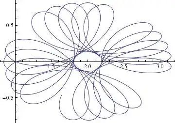
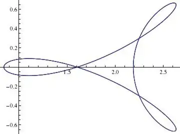
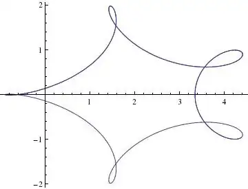
To answer the original question which asked: is it Rose, Lissajous curve or hypotrochoid?, you would have to probably properly align the final plane on which you project, so the final expression wouldn't be so messy. I haven't figured out how to do that yet.