Your equation is: $a\ln(x) + b = y$. So set up matrices like this with all your data:
$$
\begin{bmatrix}
\ln(x_0) & 1 \\
\ln(x_1) & 1 \\
&... \\
\ln(x_n) & 1 \\
\end{bmatrix}
\begin{bmatrix}
a \\
b \\
\end{bmatrix}
=
\begin{bmatrix}
y_0 \\
y_1 \\
... \\
y_n
\end{bmatrix}
$$
In other words:
$$Ax = B$$
Where
$$
A = \begin{bmatrix}
\ln(x_0) & 1 \\
\ln(x_1) & 1 \\
&... \\
\ln(x_n) & 1 \\
\end{bmatrix}
$$
$$
x = \begin{bmatrix}
a \\
b \\
\end{bmatrix}
$$
and
$$
B = \begin{bmatrix}
y_0 \\
y_1 \\
... \\
y_n
\end{bmatrix}
$$
Now solve for $x$ which are your coefficients. But since the system is over-determined, you need to use the left pseudo inverse: $A^+ = (A^T A)^{-1} A^T$. So the answer is:
$$
\begin{bmatrix}
a \\
b \\
\end{bmatrix} = (A^T A)^{-1} A^T B
$$
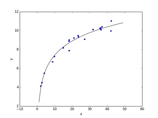
Here is some simple Python code with an example:
import matplotlib.pyplot as plt
import numpy as np

TARGET_A = 2
TARGET_B = 3
N_POINTS = 20
MAX_X = 50
NOISE_A = 0.1
NOISE_B = 0.2

# create random data
xs = [np.random.uniform(MAX_X) for i in range(N_POINTS)]
ys = []
for i in range(N_POINTS):
    ys.append((TARGET_A + np.random.normal(scale=NOISE_A)) * np.log(xs[i]) + \
              TARGET_B + np.random.normal(scale=NOISE_B))

# plot raw data
plt.figure()
plt.scatter(xs, ys, color='b')

# do fit
tmp_A = []
tmp_B = []
for i in range(len(xs)):
    tmp_A.append([np.log(xs[i]), 1])
    tmp_B.append(ys[i])
B = np.matrix(tmp_B).T
A = np.matrix(tmp_A)
fit = (A.T * A).I * A.T * B
errors = B - A * fit
residual = np.linalg.norm(errors)

print "solution:"
print "%f log(x) + %f = y" % (fit[0], fit[1])
print "errors:"
print errors
print "residual:"
print residual

# plot fit
fit_x = range(1, MAX_X)
fit_y = [float(fit[0]) * np.log(x) + float(fit[1]) for x in fit_x]
plt.plot(fit_x, fit_y, color='k')

plt.xlabel('x')
plt.ylabel('y')
plt.show()