5

I can see by manipulating the expression why $\mathbb{E}X$ works out to be $\int_0^\infty 1-F(x)\,dx$, where $F$ is the distribution function of $X$, but what is an intuitive explanation for why that is true? If at each point we sum the probability $\mathbb{P}(X>x)$, why should we end up with the expectation?

Thanks

Eric Auld
  • 28,127

2 Answers2

6

If you are looking for intuition, the discrete case is your best bet. Look at $\sum_0^\infty P[X > n]$ and count how many times you count the set $\{X = k\}$. You don't count $\{X=0\}$ at all. The only one which includes $\{X=1\}$ is $P[X>0]$ so it gets counted once. You will count $\{X=2\}$ twice, when $n=0$ and $n=1$. And so on, you will count $\{X=n\}$ exactly $n$ times.

Thus we must have $\sum_0^\infty P[X>n] = \sum_0^\infty n P[X=n] = EX$. To make the argument rigorous and also extend to the continuous case, we simply apply Fubini's Theorem (Tonelli's Theorem) to say $$ \int_0^\infty P[X>t]dt = \int_0^\infty\int1_{X>t}dPdt = \int\int_0^\infty 1_{X>t}dtdP = \int XdP = EX. $$

Edit: As Evan mentions, of course we require $X$ to be nonnegative.

nullUser
  • 27,877
  • Thank you! That is a great motivation. I am a little confused by your notation $\int_0^\infty\int1_{X>t}dPdt = \int\int_0^\infty 1_{X>t}dtdP = \int XdP = EX$, in particular the $dP$ and the $1_{X>t}$ integrating to $X$. Can you explain, or give me a reference where I can clarify my understanding here? Thanks – Eric Auld Oct 23 '13 at 15:25
  • The definition of $EX$ in general is given by a Lebesgue integral with respect to the probability measure $P$. See http://en.wikipedia.org/wiki/Expected_value under "General definition" if you are interested. Here we use the measure-theoretic foundations of probability which are much more powerful than the tools in elementary probability. However, measure theory requires some work to develop, so it is not typically taught at the undergraduate level. If you are interested in an easy introduction to measure-theoretic probability, I suggest Probability with Martingales by David Williams. – nullUser Oct 23 '13 at 15:32
  • Luckily I am familiar with measure theory, but my probability course is being taught at an elementary level. I will look at your link, thanks. – Eric Auld Oct 23 '13 at 15:44
1

This is really just another way of stating nullUser's intuitive explanation, particularly focusing on the second half (Tonelli/Fubini).

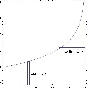
Suppose for now that our variable has the specific form $X=f(t)$, where $t$ is chosen uniformly between $0$ and $1$ and $f$ is an increasing function of $t$. In that case $E(X)$ has a natural interpretation: It just corresponds to the average value of $f$, which is just the area under $f$.

There's two ways of thinking about this area. One is "vertically", as $\int_0^1 f(t) dt$. The other is "horizontally": integrate the width of the horizontal rectangle instead of the height of the vertical one. And the width of a horizontal rectangle here just corresponds to the part of the $f(t)$ which is above $t$, i.e. the probability $X$ is at least $t$.

enter image description here

This picture was for when $X$ had this particular $f(t)$ form. For the general case, you should think of $t$ as representing a sort of percentile for $X$ (e.g. $t=0.5$ represents the median value of $X$, and $t=0.9$ a value which is only reached $10\%$ of the time). This can also be thought of in terms of a change of variables where $t=\Phi^{-1}(X)$.

  • $t=\Phi^{-1}(X)$ isn't completely accurate here (e.g. for discrete variables), but it's sort of the idea I'm trying to capture. In general, you can think of variables as coming from applying a function to a number uniformly chosen from $[0,1]$, and in this form it's sometimes easier to visualize what's going on. – Kevin P. Costello Oct 23 '13 at 20:23