$M$ in triangle $ABC$ ; images $A',B',C'$ by inversions wrt circles $(MBC),(AMC),(ABM)$ are such that $A'B'C'$ equilateral : is $M$ a known center?

Question

Yesterday, a question occurred to me, and I tried to find the center of the triangle that satisfies the condition I am thinking of, but I have not been able to do so yet

Suppose a triangle $∆ABC$, what is required is to determine the appropriate position of the point M that makes the triangle $∆A'B'C'$ To be an equilateral triangle where the points $A',B',C'$ are the inversion of the vertices of the triangle with respect to the three circles that each pass through two vertices of the triangle. And the point $M$

I tried searching some centers from the Clark Kimberling Encyclopedia online and verified that they do not achieve this property. I tried about $15 centers of the triangle. I don't want to try all the points in the encyclopedia to find this point. Is there a faster way? For example, how do we create this point with a ruler and compass?

I wrote some Mathematica code to compute the positions of $M$, given $A=(0,0)$, $B=(1,0)$ and $C=(h,k)$. I get, in general, twelve solutions, most of them complex but with 4 or 5 real solutions. No hope to get a ruler-and-compass solution, I'm afraid. — Intelligenti pauca, Feb 10 '24 at 22:42
I have attempted to propose you a more appropriate title, in order more people are attracted to your question in the future. Do you agree ? — Jean Marie, Feb 11 '24 at 12:05
@Intelligenci pauca As many as four or five in general ? I would be interested by your Mathematica code. Could you share it for example in a very simple answer ? — Jean Marie, Feb 11 '24 at 12:07
Indeed, it is a more appropriate title, @Jean Marie Thank you — زكريا حسناوي, Feb 11 '24 at 14:30

Intelligenti pauca · Answer 1 · 2024-02-11T17:23:39.060

As requested in a comment, I share in this answer some Mathematica code to compute the positions of $M$ giving an equilateral triangle.

I started with a formula for the center of the circle through three points, which I found using Mathematica (but is in fact well known): $$ x={1\over2} {x_1^2 (y_2 - y_3) +x_2^2 (y_3-y_1) + x_3^2 (y_1 - y_2) - (y_1 - y_2) (y_2 - y_3)(y_3-y_1) \over x_1 (y_2 - y_3) +x_2 (y_3-y_1) + x_3 (y_1 - y_2)} \\ y={1\over2} {y_1^2 (x_2 - x_3) +y_2^2 (x_3-x_1) + y_3^2 (x_1 - x_2) - (x_1 - x_2) (x_2 - x_3)(x_3-x_1) \over y_1 (x_2 - x_3) +y_2 (x_3-x_1) + y_3 (x_1 - x_2)} $$ Given then the vertices and point $M$ as:

a = {0, 0}; b = {1, 0}; c = {h, k}; m = {x, y};

I computed with the above formula the centers of the circles, their radii and then the inverses of the vertices:

ca = center[m, b, c]; 
ra = Sqrt[(ca - b).(ca - b)];
a1 = ca + (a - ca)*ra^2/((a - ca).(a - ca))//Simplify;

and analogous formulas for vertices $B$ and $C$. Finally, squared distances between the inverses can be computed and equated to form two equations, depending on wariables $x$, $y$, $h$, $k$. In principle one could hope to get a solution as a funcion of $(h,k)$, but I opted for the quicker option of giving a numerical value to $(h,k)$ and compute the solutions for $(x,y)$, for instance:

In[9]:= Solve[(a1 - b1).(a1 - b1) == (a1 - c1).(a1 - c1) 
        == (c1 - b1).(c1 - b1) /. {h -> 0.2, k -> 1.2}]
Out[9]= {{x -> 0.523901, y -> -0.49025}, 
         {x -> -0.120266, y -> -0.370365}, 
         {x -> 0.435031 + 0.268912 I, y -> -0.0978817 - 0.219988 I}, 
         {x -> 0.435031 - 0.268912 I, y -> -0.0978817 + 0.219988 I}, 
         {x -> 0.957536, y -> -0.0453308}, 
         {x -> 0.408247, y -> 0.348737}, 
         {x -> -0.841388, y -> 0.763081}, 
         {x -> 0.773606 - 0.543748 I, y -> 0.907342 - 0.0180481 I}, 
         {x -> 0.773606 + 0.543748 I, y -> 0.907342 + 0.0180481 I}, 
         {x -> 2.09789 - 2.49145 I, y -> 1.52241 - 1.43018 I}, 
         {x -> 2.09789 + 2.49145 I, y -> 1.52241 + 1.43018 I}, 
         {x -> 0.269251, y -> 1.62577}}

As you can see, there are 12 solutions, six of which are real. Below a figure with triangle $ABC$ and the six equilateral triangles from the above solution.

About the circle passing through 3 points, interesting methods here in particular in the answer by Scott. — Jean Marie, Feb 11 '24 at 15:08

Jean Marie · Answer 2 · 2024-02-11T11:51:44.967

It appears that $M$ can take different positions (black little circles in Fig. 1 for example) for which the result is an equilateral triangle.

Therefore, considering this issue under the point of view of "triangle centers" looks to me a dead end.

let us have a closer look. On fig. 1, a first point $M$ has been privilegized for the reproduction of the figure as given in the question. $M$, like other positions $M', M''$ are candidates obtained by a systematic "browsing", using a $400 \times 400$ grid of points of the area covering the triangle and its vicinity. It is why the displayed point(s) are close to the points realizing an equilateral triangle but not exactly coinciding with them ; as a consequence, we have a little "fuzzyness" for displayed triangles.

Fig. 1 : Triangle $A(-2,0), B(0.5,0), C(0,1)$ ; circles $(ABM),(MBC),(AMC)$ with common point $M$ in green giving light grey triangle (all this is similar to your figure). But there are two other points $M'$ and $M''$ associated resp. with purple and blue "equilateral" triangles.

Fig. 2 : (in connection with Fig. 1) ; Color display of a function characterizing "equilateralness" on a scale with minimal value $0$ (deep blue) for perfect equilateralness. One recognizes in this diagram the shape of (prolongated) triangle $ABC$ and the places where points $M,M',M''$ are situated.

Fig. 3 : Another example with an acute triangle $A=(-2,-1), B=(1,-1), C=(0,2)$ which can be seen on the upper left corner of the left figure where we can see (at least) three triangles. On the right figure one can notice three deep blue regions corresponding to these three triangles plus a whole circle which looks as a continuous locus of points $M$. Honestly, I haven't well understood all in this pretty figure.

For those who are interested, I can provide the Matlab program that I have written for obtaining this figure.

+1 Thank you very much @Jean Marie, beautiful and inspiring drawings, you are an expert in using computer software — زكريا حسناوي, Feb 10 '24 at 21:01
I just made other attempts and I realized that there are more than a single point $M$ also in the case of triangles with acute angles. — Jean Marie, Feb 10 '24 at 21:08
@JeanMarie how did you expert yourself at using such a variety of mathematics softwares? (Sage, matlab etc) — Sahaj, Feb 11 '24 at 13:15
@Sahaj Just by spending a lot of time on them for now many years... I also learned a lot by teaching programming methods to students and having their feedback... — Jean Marie, Feb 11 '24 at 13:18

Cesareo · Answer 3 · 2024-02-11T22:10:41.183

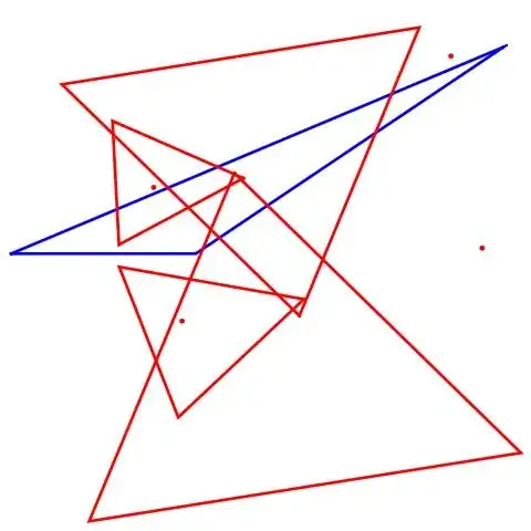
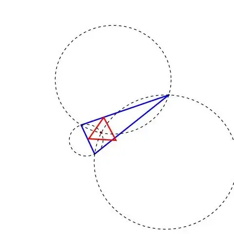
Follows a MATHEMATICA script which calculates an equilateral triangle obtained by inversion, (red) preferably when the common point to invert, (red) is located inside the original triangle (blue). There are problems of poor numerical conditioning in case of squashed triangles. Changing the value of SeedRandom[15] we can generate other base triangles.

Clear[circ]
circ[p_, p0_, r_] := (p - p0) . (p - p0) - r^2
Clear[solvecirc]
solvecirc[p1_, p2_, g_] := Module[{p0, x0, y0, equ1, equ2, equ3, sols, r0, ind, r},
  p0 = {x0, y0};
  equ1 = circ[p1, p0, r];
  equ2 = circ[p2, p0, r];
  equ3 = circ[g, p0, r];
  sols = Quiet@NSolve[{equ1 == 0, equ2 == 0, equ3 == 0}, {x0, y0, r}][[2]];
  Return[{p0, Abs[r]} /. sols];
  ]
Clear[extcirc]
extcirc[tri_, g_] := Module[{p1 = tri[[1]], p2 = tri[[2]], p3 = tri[[3]], sol1, sol2, sol3},
  sol3 = solvecirc[p1, p2, g];
  sol1 = solvecirc[p2, p3, g];
  sol2 = solvecirc[p3, p1, g];
  Return[{sol1, sol2, sol3}]
  ]
Clear[invert]
invert[g_, p0_, r_] := Module[{d},
  d = Norm[g - p0];
  Return[p0 + (g - p0) (r/d)^2]
  ]
Clear[equilat]
equilat[tri_, g_] := Module[{circs, invs, l1, l2, l3},
  circs = extcirc[tri, g];
  invs = Table[invert[tri[[k]], circs[[k, 1]], circs[[k, 2]]], {k, 1, 3}];
  l1 = (invs[[1]] - invs[[2]]).(invs[[1]] - invs[[2]]);
  l2 = (invs[[2]] - invs[[3]]).(invs[[2]] - invs[[3]]);
  l3 = (invs[[1]] - invs[[3]]).(invs[[1]] - invs[[3]]);
  Return[(l1 - l2)^2 + (l2 - l3)^2 + (l1 - l3)^2]
  ]
SeedRandom[15];
toler = 0.0001;
tri = RandomReal[{-1, 1}, {3, 2}];
regs = BoundaryDiscretizeGraphics[ListLinePlot[Join[tri, {tri[[1]]}]]];
sol = Quiet@NMinimize[{equilat[tri, {x, y}], {x, y} [Element] regs}, {x, y}, Method -> "DifferentialEvolution"]
If[sol[[1]] > toler,
 sol = Quiet@NMinimize[equilat[tri, {x, y}], {x, y}, Method -> "DifferentialEvolution"]
 ]
GRF = {};
If[sol[[1]] < toler,
 g = {x, y} /. sol[[2]];
 circs = extcirc[tri, g];
 invs = Table[invert[tri[[k]], circs[[k, 1]], circs[[k, 2]]], {k, 1, 3}];
 gr1 = ListLinePlot[Join[tri, {tri[[1]]}], PlotStyle -> Blue];
 AppendTo[GRF, gr1];
 gr2 = Graphics[{Red, PointSize[0.01], Point[g]}];
 AppendTo[GRF, gr2];
 gr4 = ListLinePlot[Join[invs, {invs[[1]]}], PlotStyle -> Red];
 AppendTo[GRF, gr4];
 gr5 = Table[Graphics[{Dashed, Circle[circs[[k, 1]], circs[[k, 2]]]}], {k, 1, 3}];
 AppendTo[GRF, gr5];
 Show[GRF, PlotRange -> {{-2, 2}, {-2, 2}}, AspectRatio -> 1], 
 Print["Out of tolerance"]
 ]

NOTE

Added some code simplifications regarding the method equilat[tri_, g_]

EDIT

Analyzing the excellent answer from @intelligenti pauca, and using the same formalism used in my previous answer, we developed a formal (algebraic) formulation which works quite well. For simplicity, the initial triangle has coordinates

$$ (0,0),(0,3),(n_x,n_y) $$

where $n_x, n_y$ are random integers in the range $(0,10)$. According to the results, we can obtain four or six solutions. Follows the script which reuses the methods already defined previously

circ[p_, p0_, r_] := (p - p0) . (p - p0) - r^2
solvecirc[p1_, p2_, g_] := Module[{p0, x0, y0, sols, r0, r},
  p0 = {x0, y0};
  sols = Solve[{circ[p1, p0, r] == 0, circ[p2, p0, r] == 0, 
                circ[g, p0, r] == 0}, {x0, y0, r}][[2]];
  Return[{p0, r^2} /. sols // Simplify]
  ]
invert[g_, p0_, r2_] := p0 + (g - p0) r2/(g - p0) . (g - p0)
g = {gx, gy};
{p12, r12} = solvecirc[{x1, y1}, {x2, y2}, g] // Simplify;
{p23, r23} = solvecirc[{x2, y2}, {x3, y3}, g] // Simplify;
{p31, r31} = solvecirc[{x3, y3}, {x1, y1}, g] // Simplify;
p1 = invert[{x1, y1}, p23, r23];
p2 = invert[{x2, y2}, p31, r31];
p3 = invert[{x3, y3}, p12, r12];
equ1 = (p1 - p2) . (p1 - p2) - (p2 - p3) . (p2 - p3);
equ2 = (p2 - p3) . (p2 - p3) - (p3 - p1) . (p3 - p1);
equ3 = (p3 - p1) . (p3 - p1) - (p1 - p2) . (p1 - p2);
SeedRandom[1];
parms = {x1 -> 0, y1 -> 0, x2 -> 3, y2 -> 0, 
         x3 -> RandomInteger[{0, 10}], y3 -> RandomInteger[{0, 10 ]}
equs = {equ1, equ3} /. parms;
solsg = Solve[equs == 0, g, Reals] // N
circs = {{p12, r12}, {p23, r23}, {p31, r31}} /. parms /. solsg // N;
points = {p1, p2, p3} /. parms /. solsg;
gs = {gx, gy} /. solsg;
gr1 = ListLinePlot[{{x1, y1}, {x2, y2}, {x3, y3}, {x1, y1}} /. parms, PlotStyle -> Blue];
gr2 = Table[ListLinePlot[Join[points[[k]], {points[[k, 1]]}], PlotStyle -> Red], {k, 1, Length[points]}];
gr3 = Graphics[{Red, PointSize[0.01], Point[gs]}];
Show[gr1, gr2, gr3, PlotRange -> All, AspectRatio -> 1, Axes -> False]

Follows a case with SeedRandom[1] which gives six solutions

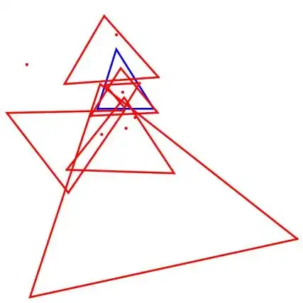
and other with SeedRandom[2] which gives four solutions

I don't understand why you consider M as the center of inversion (red point) because there are 3 centers of inversion (the circles' centers) — Jean Marie, Feb 11 '24 at 13:16

$M$ in triangle $ABC$ ; images $A',B',C'$ by inversions wrt circles $(MBC),(AMC),(ABM)$ are such that $A'B'C'$ equilateral : is $M$ a known center?

3 Answers3