2

I have modeled the interaction of two physical quantities, $S$ and $B$, by the following differential equations (the second one is a delay differential equation):

$$S'(t) = 0.31 S(t) \Big( 1 - \frac{S(t)}{6.19} \Big)- \frac{a}{1 + B(t)} S(t),$$

$$B'(t) = c (1 - B(t)) \theta(18 - t) - d B(t) S(t) - 3 c (1 - B(t - 18)),$$

where $a$, $c$, and $d$ are some constants to be determined from the experimental data and $\theta$ is the Heaviside function. The parameters are found to be: $a = 0.72$, $c = 0.19$, and $d = 0.24$; and also, the initial conditions read: $S(0) = 1.25$ and $B(0) = 1.14$.

The solutions (plotted with Mathematica) are:

Unprotect[HeavisideTheta]; HeavisideTheta[0.] = 0.5; Protect[HeavisideTheta];
so = NDSolve[{ss'[t] + 0.72/(1 + bb[t]) ss[t] - 0.31 ss[t] (1 - ss[t]/6.19) == 0, 
bb'[t] - 0.19 (1 - bb[t]) HeavisideTheta[18 - t] + 0.24 bb[t] ss[t] + 0.57 (1 - bb[t - 18]) == 0, 
ss[t /; t < 0] == 1.25, bb[t /; t < 0] == 1.14}, {ss, bb}, {t, 0, 24}];

Plot[Evaluate[bb[t] /. so], {t, 0, 24}, PlotRange -> All, AxesOrigin -> {0, 0}, PlotLabel -> "B(t)"] Plot[Evaluate[ss[t] /. so], {t, 0, 24}, PlotRange -> All, AxesOrigin -> {0, 0}, PlotLabel -> "S(t)"]

Image 1

Everything looks good, since I'm only interested in the time interval $0 < t < 24$ and the curves correctly predict the behavior of my system (experiment). However, if we simulate the differential equations further and for a larger time interval, let's say, till $t = 30$, the solutions look like:

Image 2

This is not desirable as $B$ is a physical quantity and cannot be negative.

My question is:

What kinds of terms should I add in my differential equations (or what assumptions need to be considered?) to force the $B$ solution do not cross the axis and to be bounded and remain zero at the end?

Any help is appreciated.
  • Hi Tim. I cannot deliver you an answer, but I do could tell that for simple (meaning here, not a system of equations) autonomous ODEs of first or second order, in order to have solutions with a finite extinction time they must support singular solutions (so far I understand), so they should fulfill at least this two conditions: (i) the trivial zero functions must be a solution, (ii) the differential equation must have at least one point in time were the equation is Non-Lipschitz (see this tag finite-duration). (...) – Joako Dec 11 '23 at 01:23
  • (...) But I don't know if these relations holds also for system of ODEs (maybe they need more, or less), and surely for PDEs are not required since a compact-supported solution for a wave equation, fixing the view in one point in space were the front-wave pass by, will behave as having a finite duration in time (here an example). At least in one variable, any solution through a non-piecewise power series cannot represent something that becomes exactly constant in a non-zero measure interval since will violate the Identity Theorem. – Joako Dec 11 '23 at 01:30
  • my thoughts are that since eqns are Lipschitz you wouldn't have solutions with a finite extinction time (this is true for 1st and 2nd order ODEs only, I don't know if stands for systems or neither for Delayed Diffs. eqns. which allready are "hardly" nonlinear). Try adding in the RHS of the $B(t)$ eqn a term $-a\ \text{sgn}(B'(t))$ for some real-valued constant $a>0$ to be determined. It have worked for me in other 2nd order ODEs. – Joako Dec 15 '23 at 15:27
  • 1
    Unfortunately I cannot help you much more, a few month ago I figured out these kind of solutions exists and made the tag [finite-duration] looking for answers, since I realized it have been completely ignored by the scientific community. In the tag there are some papers but I don't fully understand them (I am engineer, not a mathematician). – Joako Dec 15 '23 at 19:29
  • 1
    About your questions, the example I give you was a result of using the Coulomb friction in classic mechanics, but as you modified it I don't have an analogy. About making the equation smooth, at least for ODEs is not possible since the Non-Lipschitz point in time is required for having solutions with finite duration: I don't know if it hold for eqns. systems or DDEs, but for ODEs is explained in the papers by V.T. Haimo (on the tag page). – Joako Dec 15 '23 at 19:33
  • 1
    If you are talking about smooth functions that becomes zero and stays there, then you they don't gonna be analytic functions: check here for Non analytic smooth functions like the Bump functions. – Joako Dec 15 '23 at 19:36
  • Did you finally found an answer to your question? – Joako Dec 21 '23 at 18:31

1 Answers1

0

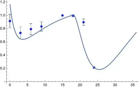
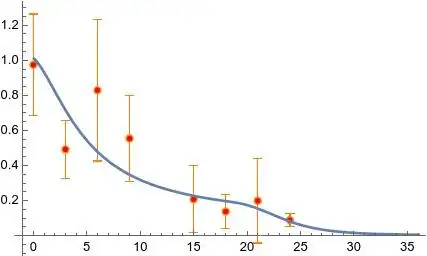
Changing the wheighting factor to k^alpha as can be depicted in the function fitness we can obtain a solution to the odes with the positive requirement.

fitness[a00_?NumberQ, c00_?NumberQ, d00_?NumberQ, s0_?NumberQ, b0_?NumberQ] := Module[{ss, bb, parms, odes, ODES, solode, cinits, ssbb, t, alpha = 1.1}, 
  odes = {ss'[t] + a00/(1 + bb[t]) ss[t] - 0.31 ss[t] (1 - ss[t]/6.19) == 0, bb'[t] - c00 (1 - bb[t]) + d00 bb[t] ss[t] + 3 c00 (1 - bb[t - 18]) == 0};
  cinits = {ss[t /; t <= 0] == s0, bb[t /; t <= 0] == b0};
  ODES = Join[odes, cinits];
  solode = Quiet@NDSolve[ODES, {ss, bb}, {t, tk[[1]], tk[[8]]}][[1]];
  Return[Sum[Norm[{y1[[k]], k^alpha y2[[k]]} - 
  Evaluate[{ss[t], k^alpha bb[t]} /. solode /. {t -> tk[[k]]}]], {k, 1, 8}]]]

tk = {0, 3, 6, 9, 15, 18, 21, 24}; y1 = {0.974, 0.492, 0.829, 0.554, 0.208, 0.138, 0.199, 0.0893}; y2 = {0.915094, 0.736097, 0.793694, 0.833664, 1, 0.99578, 0.897964, 0.214499}; SdatawithSD = {{0, Around[0.974, 0.289]}, {3, Around[0.492, 0.165]}, {6, Around[0.829, 0.404]}, {9, Around[0.554, 0.245]}, {15, Around[0.208, 0.191]}, {18, Around[0.138, 0.0962]}, {21, Around[0.199, 0.241]}, {24, Around[0.0893, 0.0359]}}; BdatawithSD = {{0, Around[0.915094, 0.1]}, {3, Around[0.736097, 0.091668]}, {6, Around[0.793694, 0.082575]}, {9, Around[0.833664, 0.070242]}, {15, Around[1, 0.002851]}, {18, Around[0.99578, 0.015591]}, {21,Around[0.897964, 0.04783]}, {24, Around[0.214499, 0.01231]}};

restrs = {0.7 - 0.2 < a00 < 1 + 0.2 && 0.1 < c00 < 0.5 + 0.2 && 0.1 < d00 < 0.5 + 0.2 && 0.9 - 0.2 < s0 < 1.2 + 0.2 && 0.9 - 0.2 < b0 < 1.2 + 0.2}; vars = {a00, c00, d00, s0, b0};

sol = Quiet@NMinimize[Join[{fitness[a00, c00, d00, s0, b0]}, restrs], vars, StepMonitor :> Print[{a00, c00, d00, s0, b0, fitness[a00, c00, d00, s0, b0]}], MaxIterations -> 10, WorkingPrecision -> 30, Method -> "DifferentialEvolution"]

odes = {ss'[t] + a00/(1 + bb[t]) ss[t] - 0.31 ss[t] (1 - ss[t]/6.19) == 0, bb'[t] - c00 (1 - bb[t]) + d00 bb[t] ss[t] + 3 c00 (1 - bb[t - 18]) == 0} /. sol[[2]]; cinits = {ss[t /; t <= 0] == s0, bb[t /; t <= 0] == b0} /. sol[[2]]; ODES = Join[odes, cinits]; solode = NDSolve[ODES, {ss, bb}, {t, tk[[1]], 1.5 tk[[8]]}][[1]];

g11 = ListPlot[SdatawithSD, PlotStyle -> {Orange, PointSize[0.02]}, AxesOrigin -> {-1, 0}]; gr10 = ListPlot[Transpose[{tk, y1}], PlotStyle -> Red, PlotLabel -> "S(t)"]; gr0 = Plot[Evaluate[ss[t] /. solode], {t, tk[[1]], 1.5 tk[[8]]}]; Show[g11, gr10, gr0, PlotRange -> All]

g22 = ListPlot[BdatawithSD, AxesOrigin -> {-1, 0}, PlotStyle -> {PointSize[0.02]}]; gr2 = ListPlot[Transpose[{tk, y2}], PlotStyle -> Blue]; gr00 = Plot[Evaluate[bb[t] /. solode], {t, tk[[1]], 1.5 tk[[8]]}]; gr02 = ListPlot[Transpose[{tk, y2}], PlotStyle -> Blue, PlotLabel -> "B(t)"]; Show[g22, gr02, gr00, PlotRange -> All]

enter image description here

enter image description here

Cesareo
  • 33,252