It is known how to compute the distribution of a product of independent random variables. The results boils down to evaluating the inverse Mellin transform of a product of Mellin transforms of the original probability densities.This approach is mentioned in the so called Slater theorem in this question and the whole theory is set out in this paper
Springer, M. D.; Thompson, W. E., The distribution of products of independent random variables, SIAM J. Appl. Math. 14, 511-526 (1966). ZBL0144.40701.
.
We used this approach to compute the result for iid, normal variables with mean zero and variance one. In other words $x= t_1 t_1 \cdots t_n$ where $t_i \sim N(0,1) $ for $i=1,\cdots,n$. Define ${\tilde x}_n:= x 2^{-n/2}$ and
\begin{eqnarray} {\mathfrak A}_m^{(n)}(x) &:=& \frac{1}{(n-1)!} \left. \frac{d^{n-1}}{d \epsilon^{n-1}} [\Gamma\left(-m+\epsilon\right) \epsilon ]^n \cdot x^{-2 \epsilon} \right|_{\epsilon=0} \\ &=& \left\{ \begin{array}{lll} \frac{(+1)^m}{[m!]^2} \left( \left\{ n \psi^{(0)}(1+m) \right\} + (-2 \log(x)) \right) & \mbox{if $n=2$}\\ \frac{(-1)^m}{[m!]^3} \left( \left\{\frac{n^2}{2!} [ \psi^{(0)}(1+m) ]^2 - \frac{n}{2!} [ \psi^{(1)}(1+m) ]^{1} + \frac{n}{3!} \pi^2\right\} + 3 \psi^{(0)}(1+m) \cdot (-2 \log(x)) + \frac{1}{2} \cdot (-2 \log(x))^2 \right)& \mbox{if $n=3$} \\ \vdots \end{array} \right. \end{eqnarray} where $\psi^{j}(\cdot)$ is the polygamma function.
For fixed $n=2,3,4,\cdots$ and arbitrary $m,x$ the quantities above can be generated using the following formula:
\begin{eqnarray} {\mathfrak A}_m^{(n)}(x) = \lim\limits_{\epsilon \rightarrow 0} \frac{(-1)^{m n}}{[m!]^n} \cdot \sum\limits_{0 \le p_1 \le p_2 \le n-1} \frac{\pi^{p_1}}{p_1! (p_2-p_1)! (n-1-p_2)!} \left(\left.\frac{d^{p_1}}{d \epsilon^{p_1}} \left( \frac{\sin(\epsilon)}{\epsilon} \right)^{-n} \right|_{\epsilon:> \pi \epsilon} \right) \cdot \left(\frac{d^{p_2-p_1}}{d \epsilon^{p_2-p_1}} \exp\left[-n \log(\frac{\Gamma(1+m-\epsilon)}{\Gamma(1+m)}) \right] \right) \cdot (-2 \log(x))^{n-1-p_2} \end{eqnarray}
Then the result reads:
\begin{equation} \rho_X(x) = \frac{2^{-\frac{n}{2}}}{\pi^{\frac{n}{2}}} \cdot \sum\limits_{m=0}^\infty \left( {\tilde x}_n \right)^{2 m} \cdot {\mathfrak A}_m^{(n)}({\tilde x}_n ) \tag{1} \end{equation}
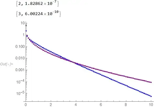
Now , by using the Mathematica code snippet below, we have plotted the result for $n=2,3$ (in Blue and Purple respectively). Here we go:
(*Distribution of a product of iid, standard Gaussian random \
variables.*)
n =.;
M = 20;
xs = Array[# &, 100, {0.001, 10}];
gamma = 0.1; Vals = {};
Do[
  Which[n == 2,
   vals1 =
     2^(-n/2)/Pi^(n/2) Total[
         Table[(# 2^(-n/2))^(2 m) ((-1)^(m n)/(m!)^2 (n) PolyGamma[0,
               1 + m] + 1/(m!)^2 (-2 Log[# 2^(-n/2)])), {m, 0,
           M}]] & /@ xs;,
   n == 3,
   vals1 = 2^(-n/2)/Pi^(n/2) Total[Table[(# 2^(-n/2))^(2 m) (
            (-1)^(m n)/(m!)^3 (1/2! n^2 PolyGamma[0, 1 + m]^2 +
                1/2! (-n)  PolyGamma[1, 1 + m] + n Pi^2/3!) +
             (3 (-1)^m PolyGamma[0, 1 + m])/
              Gamma[1 + m]^3 (-2 Log[# 2^(-n/2)]) +
             1/2 (-1)^m/(m!)^3 (-2 Log[# 2^(-n/2)])^2
            ), {m, 0, M}]] & /@ xs;
   ];
vals2 =
   2^(-1 - n/2)/
       Pi^(n/2) 1/(2 Pi ) NIntegrate[(# 2^(-n/2))^(-(gamma +
             I xi)) Gamma[(gamma + I xi)/2]^n, {xi, -Infinity,
        Infinity}] & /@ xs;
  Print[{n, Mean@Abs[vals1/vals2 - 1]}];
  Vals = Join[Vals, {vals1}];
  , {n, 2, 3}];
ListLogPlot[Transpose[{xs, #}] & /@ Vals, PlotRange :> All,
 PlotStyle :> {Blue, Purple}]
As we can see the distribution is leptokurtic with the fatness of the tail increasing with $n$. This is interesting because the Gaussian distribution does not have fat tails.
Having said all this my question would be can we generalize this approach to computing distributions of linear combinations of products of iid , standard random variables? In other words I would like to be able to compute the probability density of a a following variable $ \sum\limits_{k=0}^{n-1} {\mathfrak A}_{n,k} x_n x_{n-1-k} $ where $x_k \sim N(0,1) $ for $k=0,\cdots, n$ and $\left\{ {\mathfrak A}_{n,k} \right\}_{k=0}^{n-1}$ are some deterministic coefficients. How would we go about doing it?
