Here is an overview of how the Lebesgue integral can be reduced to the study of areas of planar diagrams. Thus perhaps surprisingly, the construction of the Lebesgue integral can be quickly reduced to a routine exercise in Riemann integration.
Given any abstract measure space $(X, \lambda)$ and a real-valued measurable function $f:X\to (0, \infty) $, define the push-forward measure $\mu=f_{*}(\lambda)$ by $\mu(I)= \lambda (f^{-1}( I))$ for every interval $I\subset (0,\infty)$.
(So for example, if the domain $X$ is say two-dimensional Euclidean space, we have used $f$ to transfer all the domain mass trapped in contour zones where $y=f(x)\in I$ onto the real axis. Our ultimate goal is to split $f$ into horizontal layers, weigh the mass of each layer, and assigned that "horizontal mass" to the vertical $y$ axis. )
The distribution function.
Define the associated distribution function of $f$ as $M_f(t) =\mu(t,\infty)$. This is essentially a cumulative distribution function; more precisely, the mass of the tail end of the real line. Distribution functions in measure theory As a function of $t$, it is monotone weakly decreasing.
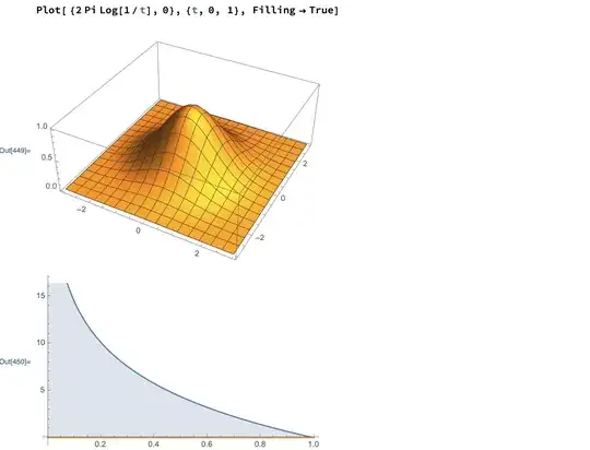
Example. It is instructive to sketch a simple special example in which we start with say $y = e^{-(x_1^2+ x_2^2)/2}$ Then a calculation shows (via the method of disks for a surface of revolution) that the distribution function is the monotone function $M_f(t) = 2\pi \ln (1/t)$ for $t<1$. As an exercise, one can check that the area under the graph of this distribution function is indeed equal to the total volume under the Gaussian function. (The distribution function redistributes mass without destroying mass.)
Exercise. A simple function is a finite sum $s(x)=\sum_k c_k i_k(x)$ where $i_k(x)$ are characteristic functions of disjoint measurable sets $E_k$ and the $c_k$ are nonnegative constants. Sketch an example of the distribution function $M_s(t)$ of a typical simple function built from say three terms. Write a formula for the area under the graph of the distribution function. Verify the non-trivial fact that the total area equals $\sum_k c_k \lambda(E_k)$.
(The point of this exercise is to confirm that the distribution function is a promising tool for defining a Lebesgue integral.)
Monotonicity properties of the distribution function
If the graph of $y=f(x)$ is truncated at tidal height $y=t$, then the dry land that lies above this tide line will shrink as the tide rises. Thus $M_f(t)$ is weakly decreasing in $t$ (order-reversing).
Lemma. If $g\leq f$ then $g^{-1}(t,\infty ) \subset f^{-1}(t,\infty)$ and $M_g(t)\leq M_f(t)$.
Thus the distribution function is weakly increasing (order-preserving) as a function of $f$.
Exercise. Use the axioms of the abstract measure space $(X, \lambda)$ and the previous lemma to show that if an increasing sequence of measurable functions $g_k\leq g_{k+1}\leq \ldots$ converges point wise to a limit function $g$, then for each fixed $t$, the sets $ E_k =g^{-1}_k( (t,\infty)$ and $E=g^{-1}( t, \infty)$ satisfy
(easy) (i) $E_k\subset E_{k+1} \ldots\subset E $ and
(less easy) (ii) $M_{g_k} (t)\uparrow M_g(t)$.
At what stage in the proof did you use the measure-theoretic properties of the measure space?
The distribution function allows us to reduce the fundamental concepts of Lebesgue integration to a much simpler context that can be treated as an elementary exercise in Riemann integration. Consider the open region $G_f$ in the first quadrant of the plane defined as all points that lie below the graph of the distribution function $y= M_f(t)$. That is, $ G_f =\{ (t, s): 0<s< M_f(t)\}$. (Here $t$ is treated as the horizontal variable.) Note that $f_1\leq f_2 \Rightarrow G(f_1)\subset G(f_2)$ (another instance of order-preserving behavior). In general the graph of the distribution function may have a vertical asymptote as $t\to 0+$ and will have a tail that decays as $t\to \infty$.
Side note. If the original measure space $X$ has unbounded total measure, then in some cases the distribution function may actually be $+\infty$ for some initial interval on the $t$ axis. To avoid this issue one commonly focuses on the class of integrable functions, defined below.
Areas of open sets
The open set $G_f$ has a well defined planar area $A(f)$, possibly infinite. There are many ways to confirm this. For example, since a monotone function has only countably many jump discontinuities, it is clear that every bounded portion of the graph has an area that can be evaluated by the Riemann method. And the total area under the graph can be defined as an improper Riemann integral, if we extend the domain of integration to the edges $t=0^+$ and $t=\infty$, so that we capture all the area under the asymptotes.
As an alternative to the Riemann integral method, one can use the dyadic square decomposition of an open set to define the area of $G$. dyadic cell decomposition
A slightly unconventional definition
Here we depart from conventional treatments of the Lebesgue integral and define the Lebesgue integral of $f$ to be the area of the region $G_f$: $$\int f d\lambda =A(G_f)$$
A nonnegative function is integrable if $A(f)<\infty$.
The Lebesgue Increasing Convergence Theorem
With this alternate definition of the Lebesgue integral, one keystone theorem in integration theory, the Lebesgue Increasing Convergence Theorem becomes a geometrically obvious property of nested open sets in the plane.
The hypotheses of the LICT are that we have an increasing sequence of nonnegative measurable functions ,
$g_k\leq g_{k+1}$
The LICT asserts that if we define $ g(x)=\lim_{k\to \infty} g_k(x)$ then $ \int g_k d\lambda \uparrow \int g d\lambda$.
That is, we can bring the limit across the integration sign.
Proof of LICT.
Pointwise we check that $g_k\uparrow g\implies g_k^{-1}(t,\infty) \uparrow g^{-1}((t,\infty))\Rightarrow M_{g_k}(t)\uparrow M_g(t)$. Thus we have the nested relations of open sets $G(g_k) \subset G(g_{k+1}) \subset G(g)$ and $G(g)=\cup_k G(g_k)$.
The regularity property of area of an increasing union of nested open sets asserts that $A(G_k)\uparrow A(\cup_kG_k)= A(G)$.
The LICT is important in measure theory because it quickly leads to a proof of the even more useful Lebesgue Dominated Convergence Theorem.
The Layer-Cake Approximation by Simple Functions
Traditionally the Lebesgue integral of a nonnegative function is defined by under-estimating $f$ by simple functions of the form $s(x)=\sum_k c_k i_k(x)$ where $i_k(x)$ are characteristic functions of disjoint measurable sets. Note that the distribution function $M_s(t)$ is just a step function whose jumps on the $t$ axis occur at the values that are sums of the $c_k$. The condition $s\leq f$ implies that $\int s d\lambda \leq \int f d\lambda$. To show that we can approximate the RHS arbitrarily well by simple functions is equivalent to arguing that the area $G_f$ can be approximated arbitrarily well by such step functions. This however is geometrically evident and is simply an easy exercise in Riemann integration.
P.S. One truly essential role of simple functions in the foundations of Lebesgue integration is that they allow us to prove the addition rule for the Lebesgue integral: $ \int (f+g) d\lambda =\int f d\lambda+ \int g d\lambda$. It is a curiosity that this "obvious" property of integration is technically more difficult to establish than the high-powered LICT ad LDCT. This is however a feature common to all treatments of the Lebesgue integral.
