Can we simplify this matrix using Vandermonde?

Question

The background has a close practical reference to (computer aided) 3D visualization techniques. It is about "melting" spheres using so-called Blinn objects (shortly "Blobs"):

For this we need a Gaussian function $g(q)=\frac{1}{\sigma\sqrt{2\pi}}e^{\frac{-|q-c|^2}{2\sigma^2}}$, $q,c\in\mathbb{R}^3,\sigma\in\mathbb{R}^+$. The Blobs are given by the set: $B_g=\{q\in\mathbb{R}^3|g_{\sigma,c}(q)=k\}$. The variable $c$ is the center of a Blob. Varying $\sigma$ adjusts the radius of a Blob. Composing these Blobs leads to a "Blobby Surface" in which the Blobs $B_i$ are melted together. For this we use the implicit functions $g_i$ and constants $k_i$:

$$ f(q)=-k+\sum_{i=1}^ng_i(q)~~\text{where}~~k=\sum_{i=1}^nk_i $$

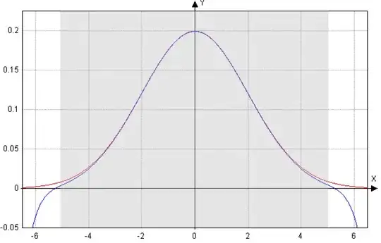
The challenge is to replace the Gaussian function by a polynom to make calculations more efficient. This can be done by approximating $g$ using a polynomial $p(x)=a_0+a_2x^2+a_4x^4+\ldots+a_{2n}x^{2n}$, where we set $p(0)=g(0)=a_0$ and $\frac{\partial}{\partial x}p(x)=\frac{\partial}{\partial x}g(x)$ for $x_1=t,x_2=2t,\ldots,x_n=nt$, $t\in\mathbb{R}^+$.

The question is: Using Vandermonde (or some similar tricks), can we simplify the resulting matrix equation that solves the coefficients of our polynomial:

$$ \begin{pmatrix} a_2\\ a_4\\ \vdots\\ a_{2n} \end{pmatrix} = \begin{pmatrix} 2\cdot(1t) & 4\cdot(1t)^3 & \cdots & 2n\cdot(1t)^{2n-1}\\ 2\cdot(2t) & 4\cdot(2t)^3 & \cdots & 2n\cdot(2t)^{2n-1}\\ \vdots & \vdots & \ddots & \vdots \\ 2\cdot(nt) & 4\cdot(nt)^3 & \cdots & 2n\cdot(nt)^{2n-1}& \end{pmatrix} \begin{pmatrix} g'(1t)\\ g'(2t)\\ \vdots\\ g'(nt) \end{pmatrix} $$

I see that the matrix structure looks a little bit like it would allow simplification using Vandermonde. Maybe there exist some tricks that enable us to benefit from Vandermonde.

For those who are interested in the approximation result (in 3D): The original "Blobby Surface" is depicted on the left and the approximated surface on the right:

$\require{HTML} \newcommand{\mypic}[4][]{ \style{ display: inline-block; background: url(https://i.stack.imgur.com/#4) no-repeat center; #1 }{\phantom{\Rule{#2}{#3}{0px}}}}$

$$\begin{array}{cc} \mypic{280px}{300px}{4lD4xm.png}& \mypic{280px}{300px}{cmNLWm.png} \end{array}$$

The approximation of the Gaussian curve (red) by the polynomial (blue) looks as follows:

Answer 1

The coefficient matrix $M$ of entries $$ M_{ij}=(2j)(it)^{2j-1},\qquad i,j=1,\dots,n, $$ can be factorized as $$ M=diag(2,4,\dots,2n)V(1,4,\dots,n^2)diag(2t,(2t)^3,\dots,t^{2n-1}) $$ where $V(x_1,\dots,x_n)$ is the Vandermonde matrix, with entries $V(x_1,\dots,x_n)_{i,j} = x_i^{j-1}$.

Thus to invert $M$ it is enough to invert the particular Vandermonde matrix $V(1,4,\dots,n^2)$. There are general formulae for the inverse of $V(x_1,\dots,x_n)$, though I do not know if they give anything explicit in this case.

Answer 2

This is more a comment, but I lack the reputation to comment; intended to help find pertinent background information and understanding.

The generalization of Blinn objects are metaballs, where the Gaussian function $g()$ is replaced by an arbitrary real function; most typically a function of the distance to the center of each metaball component.

The most generic form for a metaball is $$\sum_k g(x, y, z, x_k, y_k, z_k, w_k) \le C \tag{1}\label{BtV1}$$ where $x_k, y_k, z_k$ is a vector referring to the center of metaball component $k$, $w_k$ is the weight factor of said component, and $C$ is the isosurface threshold. ($\eqref{BtV1}$ is true for the volume within the metaball; for the isosurface, the sum equals $C$.)

Typical form used in computer graphics is $$\begin{aligned} g(x, y, z, x_k, y_k, z_k, w_k) &= w_k f(r_k^2) \\ r_k^2 &= (x - x_k)^2 + (y - y_k)^2 + (z - z_k)^2 \\ \end{aligned}$$ with $f(r_k^2) = r_k^{-4}$ (i.e. $f(x) = 1/x^2$) being a common choice.

Sometimes different support functions $f$ are used, so that the metaball equation used is actually $$\sum_k w_k f_k(r_k^2) \le C$$

The reason squared distance is used, is that the square root operation is computationally relatively expensive, and using integer powers of distance squared avoids that, yielding a computationally more efficient (faster) object evaluation.