The answer by heropup is correct in the sense that, yes, the ranges t=-100..100 will overlap many times. That's because the period of r(t) is only 2*Pi.
The situation with t=0..8*Pi is similar, but with less overlap.
But it is not true that the plot3d command will choose the points according to some algorithm that relies on continuity and smoothness. Your r(t) is smooth and continuous. It is not true that it "...chooses some points that it thinks are representative of the behavior of the curve".
A more correct explanation is that there is no adaptive sampling algorithm at work here. Rather, the problem arises because the points are taken by a uniform splitting of the range into (default) 49 values for each of the two parameters. You have only one parameter, t, and the other is taken as some dummy.
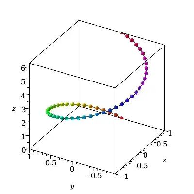
It helps to visualize what's going on if we add a vertical z-component, to show the curve as a spiral.
restart:
with(VectorCalculus):
ihat := <1, 0, 0>:
jhat := <0, 1, 0>:
khat := <0, 0, 1>:
P:=plot3d(cos(t)*ihat + sin(t)*jhat + t*khat,
          t = 0..2*Pi,
          style=pointline, symbol=solidcircle, symbolsize=20,
          color=t, orientation=[-150,60,0], labels=[x,y,z]):
P;
The data points are stored in the plotting structure (assigned to P here) in a 49x49x3 Array. Here are the dimensions on that Array.
op(2,op([1,1],P));
  1 .. 49, 1 .. 49, 1 .. 3
Even here there is waste, as there are 49 duplicates x-y-z triples stored (because of the unseen dummy 2nd parameter which takes on 49 unused values) for each of the 49 t-values.
We could greatly reduce the storage by forcing the dummy 2nd parameter's resolution to be just 2, the minimal allowed for the plot3d command. We get the same curve as before, but using far less storage, ie. roughly only 2/49 times the earlier storage.
plot3d(cos(t)*ihat + sin(t)*jhat + t*khat,
       t = 0..2*Pi, grid=[49,2],
       style=pointline, symbol=solidcircle, symbolsize=20,
       color=t, orientation=[-150,60,0], labels=[x,y,z]);

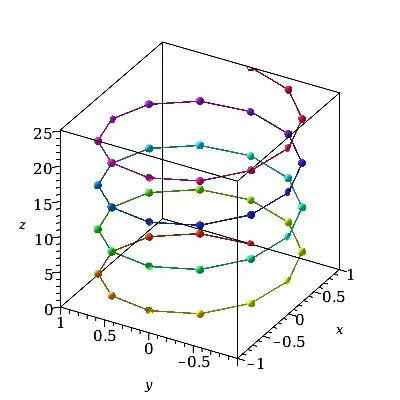
Here is the case for t=0..8*Pi. Since that has to split this wider t-range into the same default number of only 49 t-values the granularity of the t-resolution becomes more apparent.
plot3d(cos(t)*ihat + sin(t)*jhat + t*khat,
       t = 0..8*Pi,
       style=pointline, symbol=solidcircle, symbolsize=20,
       color=t, orientation=[-150,60,0], labels=[x,y,z]);
As user64494 mentions, you can correct for this (if you really insist on an unnecessarily wide t-range which entails overlapping) by specifying a larger resolution for the t-parameter. But you really should not also specify the resolution for the dummy second parameter as 600, as user64494 suggested in code. That would consume even more wasted storage. (As seen above, you can also save much wasted space by specifying the unseen dummy parameter's resolution to the minimal allowed which is 2.)
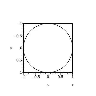
You could even get fancy in trying to guess-timate how many t-values might look ok...
G:=ceil((100+100+1)/(2*Pi))*49;
        G := 1568


plot3d(cos(t)ihat + sin(t)jhat, t = -100 .. 100,
       grid = [G, 2],
       labels=[x,y,z], orientation=[90,0,-180]);
Even this involves twice as much storage as necessary, because of the dummy second parameter. The easiest way to further halve the storage is to use instead the spacecurve command, which uses only one parameter (ie. no dummy 2nd parameter at all). Eg,
PS:=plots:-spacecurve(cos(t)*ihat + sin(t)*jhat,
                      t = 0..2*Pi,
                      color=black, orientation=[-150,60,0],
                      labels=[x,y,z]);
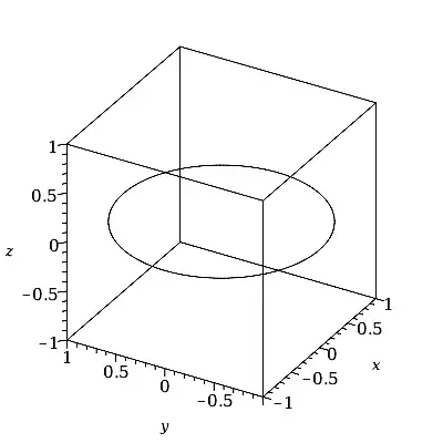
That uses 200 t-values by default. The Array which stores the data has one less dimension.
op(2,op([1,1],PS));
    1 .. 200, 1 .. 3
And you can raise that (if for some reason you insist on a range much wider than the period). Eg, with another guess-timate,
plots:-spacecurve(cos(t)*ihat + sin(t)*jhat,
                  t = -100..100, numpoints=ceil((100+100+1)/(2*Pi))*49,
                  color=black, orientation=[-150,60,0],
                  labels=[x,y,z]);


