How do I determine the function of a cardioid-like curve based on its given tangents?

Question

First of all, everything that follows refers to real functions and numbers. Let us define a parametric equation $r(t)=(x(t),y(t))=(-\sin{t},\cos{t})$ and two functions: \begin{equation*} f(x)=4x\qquad\text{and}\qquad g(x)=\frac{x}{2^{\lfloor\ln(x)\rfloor}} \end{equation*}

We retrieve the tangents by iterating $t$ within a real interval $]0,stop]$, where each tangent passes the two points $P_1$ and $P_2$:

\begin{array}{ll} P_1=(x_{P_1},y_{P_1})=r(2\pi\cdot g(t))) & P_2=(x_{P_2},y_{P_2})=r(2\pi\cdot g(f(t))) \end{array}

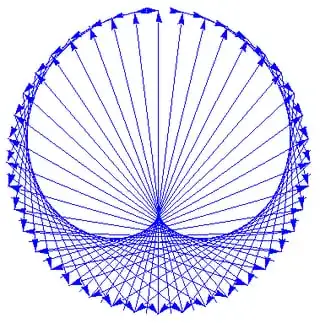
For example, when $t$ ran from $1$ to $100$ in steps of $0.2$ we retrieve the following cardioid-like curve:

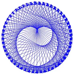
Many such curves can be generated by varying the functions $f$ and $g$ slightly, for example:

How can I proceed to determine the function of these nice curves from its given tangents resulting from the parameterized equation $r(t)$ and both functions $f$ and $g$?

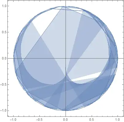
One can retrace and plot the curve as a family of lines using the following parametric function:

r[t_] := (x = -Sin[t]; y = Cos[t]; {x, y});
f[n_] := n*4;
g[n_] := n/2^Floor[Log[n]];
parametricFunc[t_, u_] := (P1 = r[2 Pi*g[t]]; 
   P2 = r[2 Pi*g[f[t]]]; {P1[[1]] + u*(P2[[1]] - P1[[1]]), 
    P1[[2]] + u*(P2[[2]] - P1[[2]])});
ParametricPlot[parametricFunc[t, u], {t, 0.01, 1}, {u, 0, 1}]

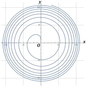
It produces the following definition:

Maybe https://en.wikipedia.org/wiki/Caustic_(optics) is of help. — Michael Hoppe, May 30 '21 at 08:41
Maybe it is solvable by the use of tangent bundles (https://en.wikipedia.org/wiki/Tangent_bundle)? It seems to be a taks of doing an integral. — , May 30 '21 at 09:04
FYI, your $g$ simplifies to $g(x)=\dfrac{x}{2^{\lfloor \ln x\rfloor}}$, since $2^{k+1}-2^{k}=2^{k}(2^1-1)=2^{k}\cdot 1$. — Blue, May 30 '21 at 13:29
The term-of-art for the curve tangent to a family of lines is the envelope of those lines. The method of determining the equation is pretty straightforward in theory (eliminate parameter $t$ from the defining relation and its derivative), but can be tricky in practice as the system could be transcendental. — Blue, May 30 '21 at 13:35
@Blue: Thank you very much for your hints. The simplification is really helpful as well as the direction to envelopes, which I will investigate. I just ordered Bruce & Giblin's book "Curves and Singularities". — , May 30 '21 at 15:16
@EldarSultanow: Does(n't) your first curve actually use $f(x)=2x$ (instead of $4x$)? — Blue, May 30 '21 at 23:31
@Blue: I just checked it and can confirm that the first curve is actually using $f(x)=4x$. The last curve (the one with the heart) is for example using $f(x)=3x$ and $g(x)=\frac{x}{2^{\lfloor\ln(x)\rfloor}}$ — , May 31 '21 at 04:32
This I had not on my radar. It would be great if I may use this simplification to calculate the envelope. Can I just use $g(x)=\frac{1}{x}$? — , May 31 '21 at 05:57
@EldarSultanow: Hmm ... I can't (yet) tell why either of us would be off by a factor of $2$. ... Here's where I am on this: $\lfloor\ln x\rfloor$ over successive intervals $I_k:=[e^k,e^{k+1})$ (for integer $k$) is constant (namely, $k$). Writing, say, $f(x)=ax$, we have $g(f(x))=2^{-k}\cdot ax=a\cdot g(x)$ on $I_k$. This implies $P_2$ moves around the circle at $a$-times the speed of $P_1$ (for each $k$!). It is "known" (and readily proven) that the resulting envelope is a cardioid when $a=2$; your first image even appears to illustrate this. ... Perhaps I'll see the error after a break. — Blue, May 31 '21 at 06:57
@Blue: Obtaining a formula for this curve would be great. I tried to set first derivative equal to zero and resolve to $t$ - without success (it is a very complicated term involving $\sin$ and $\cos$ functions). Where do I find the prove that the resulting envelope is a cardioid? If you need anything (pieces of code Mathematica / Python ore more examples), let me know. — , May 31 '21 at 08:24
Maybe using the sawtooth function instead of floor helps us to get the derivative? I found this post that maybe helps: https://math.stackexchange.com/questions/2746958/smooth-floor-function — , May 31 '21 at 11:24
@EldarSultanow: See Wikipedia's "Cardioid" entry, under Cardioid as a pencil of lines. (Note that the text there observes "The second point [of the two defining the chord tangent to the curve] is moved by double velocity", which is consistent with my comment about $a=2$.) — Blue, May 31 '21 at 12:06
ok - I checked my notebook and replaced $4$ with $2$ and as you said I get also a cardioid. So both factors work. — , May 31 '21 at 12:41
@EldarSultanow: I've identified my problem as not paying careful-enough attention to when values jump those $I_k$ intervals I defined. Interval-jumping affects whether the relation $g(ax)=a\cdot g(x)$ holds. ... So, the situation isn't quite as clean-cut as I seem to have indicated. Subdividing the intervals appropriately should rectify the situation, but I'll need to give that a little more thought. — Blue, May 31 '21 at 14:22
We need to resolve $t$ in $\frac{\partial F}{\partial t}(x,y,t)=2\pi\left(\frac{4}{2^{\lfloor\ln{4t}\rfloor}}\left(\cos{\left(\frac{2\pi t}{2^{\lfloor\ln{t}\rfloor}}-\frac{2\pi t\cdot4}{2^{\lfloor\ln{4t}\rfloor}}\right)}-y\cos{\frac{2\pi t\cdot4}{2^{\lfloor\ln{4t}\rfloor}}}+x\sin{\frac{2\pi t\cdot4}{2^{\lfloor\ln{4t}\rfloor}}}\right)-\frac{1}{2^{\lfloor\ln{t}\rfloor}}\left(\cos{\left(\frac{2\pi t}{2^{\lfloor\ln{t}\rfloor}}-\frac{2\pi t\cdot4}{2^{\lfloor\ln{4t}\rfloor}}\right)}-y\cos{\frac{2\pi t}{2^{\lfloor\ln{t}\rfloor}}}+x\sin{\frac{2\pi t}{2^{\lfloor\ln{t}\rfloor}}}\right)\right)$ — , Jun 01 '21 at 16:18
@Blue: I could follow your idea: The following equality holds for $x\in I_k$ and two functions $g_1(x)=\frac{x}{2^{\lfloor\ln{x}\rfloor}}$ and $g_2(x)=\frac{x}{2^k}$: $g_1(x)=g_2(x)$ and $g_1\circ f_a(x)=g_2\circ f_{\frac{a}{2}}(x)$. We still need to restrict $a$ as follows: $\lfloor\ln{a}+\ln{x}\rfloor=k+1$ respectively $e\le a<e^2$. And the equation becomes $F(x,y,t)=(y+1)\sin{(\pi t)}-y\sin{(2\pi t)}+x\cos{(\pi t)}-x\cos{(2\pi t)}=0$ — , Jun 05 '21 at 22:54
@EldarSultanow: That may be correct; I haven't checked. ... Ultimately, your curve appears to be the union of cardioid-like envelopes of chords whose endpoints traverse the circle at different (but individually-constant) rates. The specific rates, and extents of arcs, depend upon the subdivided $I_k$ intervals. The whole thing is a bit of a mess near zero (where there are infinitely-many tiny intervals); also, using a base-$e$ log as an exponent on $2$ just adds to the mess. I'm afraid my enthusiasm for sorting-out the nuances of this curiosity has evaporated, but I wish you luck. Cheers! :) — Blue, Jun 06 '21 at 00:18
Thank you a lot - I have now a direction to investigate further. — , Jun 06 '21 at 08:26

Narasimham · Answer 1 · 2021-05-31T15:04:33.030

0

Could not quite understand how the curve is defined.

The following includes a drastic simplification of $g(t)$ using identity

$$ u ^ {\log v} = v^ {\log u} ; \; $$

$$f(t)=4t$$ $$g(t)=\frac{t}{2^{\log t}}=\frac{t}{t^{\log 2}}= t^ \lambda \text{ if}\;\lambda= (1- \log 2) $$ $$ g(f(t))= (4t)^\lambda $$

Connecting vector $ ( P1-P2) $ parametrization

$$ 2 \pi(4^\lambda -1) (-\sin t,\cos t)\; t^\lambda; \;$$

which plots to a spiral $(0<t< 50) $ before even going to its envelope.

Please comment for further understanding of the question.

edited May 31 '21 at 15:04

answered May 30 '21 at 20:56

Narasimham

40,495

The curve can be understood as a family of lines. I do not get a spiral but I can provide you the parametric function and its plot. For this I extend my question to add a picture. Just a moment. – May 31 '21 at 04:39
Thank you very much for your help. In order to make it more retracable I added a small snippet (Mathematica) containing four lines of code that specify and plot the parametric function. – May 31 '21 at 04:50
When I remove the floor operation from $g(x)$, I get the spiral too. – May 31 '21 at 05:32

How do I determine the function of a cardioid-like curve based on its given tangents?

1 Answers1