How can two seemingly identical conditional expectations have different values?

Question

Background

Suppose that we are using a simplified spherical model of the Earth's surface with latitude $u \in (-\frac {\pi} 2, \frac {\pi} 2)$ and longitude $v \in (-\pi, \pi)$. Restricting attention to the hemisphere, $H$, where $u, v \in (-\frac {\pi} 2, \frac {\pi} 2)$, a simple map projection from $H$ can be obtained by just taking the $x$ and $y$ coordinates via $x = \cos u \sin v$ and $y = \sin u$, which is a smooth one-to-one transformation on $H$. Now, picking a point with coordinates $(U, V)$ on $H$ uniformly according to surface area, the joint density of $U$ and $V$ is $$f_{U, V}(u, v) = \frac 1 {2\pi} \cos u, \quad \lvert u \rvert, \lvert v \rvert < \frac {\pi} 2.$$

Question

$(a)\quad$ Find $\mathbb{E}[\lvert \sin U \rvert \mid V = 0]$.

$(b)\quad$ Find $\mathbb{E}[\lvert Y \rvert \mid X = 0]$.

$(c)\quad$ Observe that $\lvert Y \rvert = \lvert \sin U \rvert$ and the event $\{X = 0\}$ is exactly the same as the event $\{V = 0\}$. How is it possible that $\mathbb{E}[\lvert Y \rvert \mid X = 0] \neq \mathbb{E}[\lvert \sin U \rvert \mid V = 0]$?

My working

I have omitted intermediate steps and only shown the essential parts to minimise the length of this post.

$(a)$

$$\begin{aligned} \because f_{U \mid V = v}(u) & = \frac 1 2 \cos u,\quad \lvert u \rvert, \lvert v \rvert < \frac \pi 2 \\[5 mm] \therefore \mathbb{E}[\lvert \sin U \rvert \mid V = 0] & = \int^{\infty}_{-\infty} \lvert \sin u \rvert \left(\frac 1 2 \cos u\right)\ \mathrm{d}u \\[5 mm] & = \int^{\frac \pi 2}_0 \sin u \cos u\ \mathrm{d}u \\[5 mm] & = \frac 1 2 \end{aligned}$$

$(b)$

$$\begin{aligned} \\[5 mm] \because f_{X, Y}(x, y) & = \frac 1 {2 \pi \sqrt{1 - y^2 - x^2}}, \quad x^2 + y^2 < 1 \\[5 mm] \therefore f_{Y \mid X = x}(y) & = \frac {\frac 1 {2 \pi \sqrt{1 - y^2 - x^2}}} {\int^{\sqrt{1 - x^2}}_{-\sqrt{1 - x^2}} \frac 1 {2 \pi \sqrt{1 - y^2 - x^2}}\ \mathrm{d}y} \\[5 mm] & = \frac 1 {\pi \sqrt{1 - y^2 - x^2}}, \quad x^2 + y^2 < 1 \\[5 mm] \implies \mathbb{E}[\lvert Y \rvert \mid X = 0] & = \int^{\infty}_{-\infty} \frac {\lvert y \rvert} {\pi \sqrt{1 - y^2}}\ \mathrm{d}y \\[5 mm] & = \frac 2 \pi \int^1_0 \frac y {\sqrt{1 - y^2}}\ \mathrm{d}y \\[5 mm] & = \frac 2 \pi \end{aligned}$$

$(c)\quad$ Although $\lvert Y \rvert = \lvert \sin U \rvert$ and the event $\{X = 0\}$ is indeed identical to the event $\{V = 0\}$, we must be mindful of the coordinate systems in play here. In particular, there are two - the $(x, y)$ plane and the $(u, v)$ plane, which are not identical but related by a transformation. Thus, since $\lvert Y \rvert$ and the event $\{X = 0\}$ concern the $(x, y)$ plane, while $\lvert \sin U \rvert$ and the event $\{V = 0\}$ concern the $(u, v)$ plane, it follows that $\mathbb{E}[\lvert Y \rvert \mid X = 0] \neq \mathbb{E}[\lvert \sin U \rvert \mid V = 0]$.

---

I think my answers to $(a)$ and $(b)$ are correct, but I am not sure about my answer to $(c)$, so any intuitive explanations will be greatly appreciated!

Answer 1

How is it possible that $\mathbb{E}[\lvert Y \rvert \mid X = 0] \neq \mathbb{E}[\lvert \sin U \rvert \mid V = 0]$?

The "ratio definition" of conditional probability densities for continuous distributions (which you're using to determine the conditional expectations) involves a certain limit: $$\begin{align}f_{Y\mid X}(y\mid x)&:={\text{d}\over \text{d}y}\lim_{\epsilon\,\downarrow\,0}P(Y\le y\ \pmb{\mid}\ x-\epsilon<X<x+\epsilon)\tag{1}\\[3mm] &=\frac{f_{X,Y}(x,y)}{f_{X}(x)}\ \ \text{when}\ f_{X}(x)>0.\tag{2} \end{align}$$ where $\{x-\epsilon<X<x+\epsilon\}\,\downarrow\,\{X=x\}$ as $\epsilon\downarrow 0.$ (E.g., see Ash, "Probability and Measure Theory", 2nd ed., pp. 206-207.)

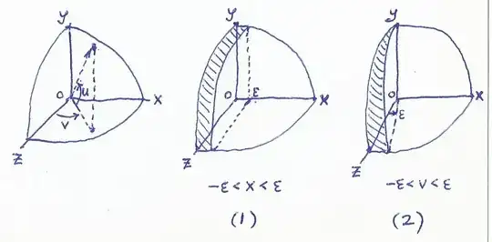
In the present problem, we're contrasting quantities defined by two different convergent sequences of sets, even though these sequences are not explicit in the notation. The key point is that although the limit events $\{X=0\}$ and $\{V=0\}$ are equivalent, the sequences converging to them are not:

(1) $E(|Y|\mid X=0)=\int_{\mathbb{R}} |y|f_{Y\mid X}(y\mid x) dy=2/\pi.$ In this case, the sets converging to $\{X=0\}$ are of form $\{-\epsilon<X<\epsilon\},$ carving from the hemisphere thin half-disks.

(2) $E(|Y|\mid V=0)=\int_{\mathbb{R}} |y|f_{Y\mid V}(y\mid v) dy=1/2.$ In this case, the sets converging to $\{V=0\}$ are of form $\{-\epsilon<V<\epsilon\},$ carving from the hemisphere thin wedges.

Here are some exaggerated sketches showing just one octant:

Some intuition: Since the distribution is uniform on the surface of the sphere, the wedge-shape (2) will --compared to (1)-- give more weight to the smaller $|y|$-values near the "equator" and less weight to the larger $|y|$-values near the "poles", so we expect to find $E(|Y|\mid X=0)>E(|Y|\mid V=0)$, which is indeed the case.

---

More generally, suppose we have a well-behaved transformation from $(X,Y)$ to $(V,Y)$, where $V=g(X,Y)$. It's then straightforward to see how the density-ratios transform: The conditional densities are related via the Jacobian of the transformation, as follows (writing "$\propto$" to omit any factors not depending on $y$):

$$\begin{align} f_{Y\mid X}(y\mid x) &\propto f_{X,Y}(x,y)\\ &\propto f_{V,Y}(g(x,y),y)\left|{\partial(v,y)\over\partial(x,y)}\right|\\ &\propto f_{V,Y}(g(x,y),y)\left|{\partial g\over\partial x}\right|\\ f_{Y\mid X}(y\mid x)&\propto f_{Y\mid V}(y\mid g(x,y))\,f_V(g(x,y))\left|{\partial g\over\partial x}\right|\\ \end{align}$$ So if we have equivalent events $\{X=x_0\}=\{V=v_0\}$, then $g(x_0,y)=v_0$, and $$\begin{align} f_{Y\mid X}(y\mid x_0) &\propto\ f_{Y\mid V}(y\mid v_0)\,\left|{\partial g\over\partial x}\right|_{x=x_0}\\[2ex] \therefore\ \ f_{Y\mid X}(\cdot\mid x_0)\ &\ \color{blue}{\ne}\ f_{Y\mid V}(\cdot\mid v_0)\\[2ex] \therefore\ \ \mathbb{E}[h(Y)\mid X=x_0]\ &\ \color{blue}{\ne}\ \mathbb{E}[h(Y)\mid V=v_0] \end{align}$$ assuming the Jacobian factor is not free of $y$ when evaluated at $x=x_0$. (E.g., in the OP's problem, $v=g(x,y)=\sin^{-1}({x\over\sqrt{1-y^2}})$, so $\left|{\partial g\over\partial x}\right|_{x=x_0=0}=1/\sqrt{1-y^2},$ hence $f_{Y\mid X}(\cdot\mid 0)\ne f_{Y\mid V}(\cdot\mid 0).$

---

NB: The use of conditional densities as density-ratios without regard to the limit process on which they depend, seems to be a perfect example of the prescription in Jaynes (2003) (p. 485) for "How to mass-produce paradoxes":

(1) Start from a mathematically well-defined situation [...] where everything is well-behaved [...] (2) Pass to a limit [...] without specifying how the limit is approached. (3) Ask a question whose answer depends on how the limit was approached.

---

Re: your other questions ...

The hemisphere $H$ is symmetrical about the positive $z$-axis, and the coordinate transformation equations are as given by the OP: $$\begin{align} X&=\cos U\sin V\\[2ex] Y&=\sin U \end{align}$$ whose inverse is $$\begin{align} U&=\sin^{-1}Y\\[2ex] V&=\sin^{-1}\left({X\over\sqrt{1-Y^2}}\right). \end{align}$$

Now, the element of area on $H$ is $dA = \cos u\,du\,dv$, from which we can derive the joint density function $f_{U,V}(u,v)$ for a uniform distribution on $H$: $$f_{U,V}(u,v)\,du\,dv= {1\over {1\over 2}(4\pi)}dA={1\over 2\pi}\cos u\,du\,dv $$ hence $$f_{U,V}(u,v)={1\over 2\pi}\cos u\,(-\pi/2<u,v<\pi/2).$$

Using this, I verified all of the OP's results, finding the joint, marginal, and conditional probability densities, and the conditional expectations.

It seems worth mentioning that $(U,V)$ are independent but not both are (marginally) Uniform, whereas $(X,Y)$ are not independent but both are (marginally) Uniform.

Answer 2

Suppose we have a bivariate normal random variable with parameters $(\mu_1, \mu_2, \sigma_1^2, \sigma_2^2,\rho)$ being $(X,Y)\sim\text{Bivariate Normal}(1,2,1,1,\frac 12)$. From properties of bivariate normals we know that $X|Y\sim\text{Normal}(\frac y 2,\frac 34)$. Let $U=X+3,V=3Y$ and let's see what happens when we condition on a probability zero event in the first "coordinate system" and the second one. The pdf of $(U,V)$ can be found to be $\text{Bivariate Normal}(4, 6, 1, 3^2, \frac 12)$. So we again can get the conditional distribution $U|V\sim \text{Normal}(\frac v 6+3, \frac 34)$. Now note that $U=X+3$ so we can try $U^2=(X+3)^2$ and the event $\{Y=1\}$ is the same as the event $\{V=3\}$, though both undoubtedly have probability zero. But then $E(U^2|V=3)=13=E((X+3)^2|Y=1)$.

Believing that this might be due to conditioning on the same "shape", e.g. in the Wikipedia article it is said that conditioning on lunes and wedges would produce different results, but here we only had two bivariate normals, in fact with the same $\rho$ parameter, so it could be possible that $\{V=3\}$ and $\{Y=1\}$ are similar cross sectional volumes.

I tried again with a different example. $f(x,y)=e^{-x}, 0<y<x<\infty$ This has conditional distribution $f(x|y)=e^{y-x}, x>y>0$ and used the transformation $U=3X,V=\frac Y3$. This has joint distribution $g(u,v)=e^{-\frac u3}$ and conditional distribution $g(u|v)=\frac 13 e^{-\left(\frac u3+3v\right)}$. $U=3X$ as defined and the event $\{Y=3\}$ is the same as $\{V=1\}$. So trying again

$$E(3X|Y=3)=\int_3^\infty e^{3-x}xdx=12\\ E(U|V=1)=\int_9^\infty \frac 13e^{\left(\frac u3-3\right)}udu=12$$

which are still the same. Looks like we will need a better transformation.

Answer 3

You can write both conditional expectations as limits of conditioning on $V\in[-\epsilon, \epsilon]$ and $Y\in [-\epsilon, \epsilon]$, respectively. Visualize these two areas for yourself and convince yourself that the corresponding limits zoom into different areas of the hemisphere (the latter area being consistently larger than the former/containing an area by the poles not covered by the former).

Basically the only reason the actual limit sets are the same is that you have an open domain rather than a closed one, so the part on the poles of the Y limit disappears in the limit, but the conditional expectation doesn't care for that unnatural disappearance.