The $\underline{\text{Riemann zeta}}$ $ \zeta (s) $ function is defined in the region $ \Re (s)> 1 $ by the convergent series
$$ \zeta(s)=\sum_{n=1}^{\infty}\frac{1}{n^{s}}=1+\frac{1}{2^s}+\frac{1}{3^s}+\dots \tag{1} $$
For $ \Re (s) \le 1 $, the series is no longer convergent, however $ \zeta $ can be extended into this region via $\underline{\text{analytic continuation}}$. This allows us to assign a value to $ (1) $ even when it would formally diverge. For example, after analytic continuation, we have $ \zeta (0) = - 1/2 $ and $ \zeta (-1) = - 1/12 $.
We will therefore show the link between the value obtained from the analytic continuation of $ \zeta $ and the limit $ N \to \infty $ of $ \sum_ {n = 1} ^ N 1 / n^s $. We will then clarify why the statement "the sum of all natural numbers equals $ -1 / 12 $" is wrong and why this misunderstanding exists.
$$ 1 + 2 + 3 + \dots \neq- \frac {1} {12} = \zeta (-1). $$
Classically a value is assigned to "infinite sums" (converging or diverging) as the result of an arithmetic operation applied infinite times. A value obtained after analytical continuation is instead linked to a complex analysis operation that cannot be obtained from the repetition of arithmetic operations on natural numbers. The values obtained through the infinite application of arithmetic operations and the values obtained through analytical continuation are however linked and in some cases may coincide. For this we will make the example of the $ \underline {\text {Casimir effect}} $.
$ \ $
$$\underline{\text{Basic knowledge, informally expressed}}$$
Indicator Function The indicator function of a subset $ A $ of $ X $ is a function
$$ \mathbb{1}_A:X\to \{0,1\} $$
defined as
$$ \mathbb{1}_A(x) =
\begin{cases}
1 & \text{if }x \in A \\
0 & \text{if } x \notin A
\end{cases} $$
Eg. $\mathbb{1}_{[0,1]}(x)$ is a function that returns $ 1 $ for all $ 0 \le x \le 1 $ otherwise $ 0 $.
Cutoff function A cutoff function is defined as a $ \eta: \mathbb {R} \to \mathbb {R} $ function such that
$$\eta \in C^{\infty}(\mathbb{R}) \ \ \ \ \eta=\begin{cases}
1 & \text{if }|x|\le 1 \\
0\le \eta(x) \le 1 & \text{elsewhere} \\
0 & \text{if } x \ge 1+\epsilon
\end{cases}$$
For our purposes the $ \eta (x) $ function is "smoother" indicator function. $ \eta (x) $ is a $\underline {\text{Schwartz function}}$.
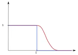
Example to compare an indicator function (blue) with a cutoff function (red)
$ \ $
- Schwartz function A function $ f\in C^{\infty} ( \mathbb{R}^n) $ is a Schwartz function if it goes to zero when $ | x | \to \infty $ faster than any inverse power of $ x $ ($ x ^ {1 / n} $), as well as its derivatives.
That is: $ f \in \mathcal {S} (\mathbb {R} ^ n) $ if there exists a constant $ C _ {\alpha, \beta} $ such that
$$\underset{x \in \mathbb{R}^n }{\sup}|x^{\alpha}\partial^{\beta}f(x)|\le C_{\alpha, \beta} $$
where $ \alpha, \beta $ are $\underline {\text{multi-index}}$.
Fourier transform The Fourier transform of a Schwartz function is still a Schwartz function denoted by $ \hat {f} (t) $ defined as
$$ \hat{f}(t) = \frac{1}{2 \pi}\int_{\mathbb{R}} f(x) e^{ i t x} dx$$
by the $\underline {\text{Fourier inversion theorem}}$
$$ f(x) = \int_{\mathbb{R}} \hat{f}(t) e^{- i t x} dt.$$
Holomorphic and meromorphic functions A holomorphic function is a complex function that can be differentiated (in a complex sense) at any point of the set on which it is defined.
A meromorphic function is a holomorphic function on the whole set on which it is defined with the exception of a set of isolated points which are the $\underline {\text{poles}}$ of the function itself.
Pole The pole of a meromorphic function $ f (z) $ is an isolated singularity $ z_0 $ such that
$$ \lim_{z \to z_0} |f(z)|= +\infty.$$
The $\underline {\text{order of the pole}}$ is a natural number $ m> 0 $ such that if $ z_0 $ is a pole, the limit
$$ \lim_{z \to z_0} f(z)(z-z_0)^m $$
exists, is finite and is not equal to 0. If $ m = 1 $, $ z_0 $ is called $\underline{\text{simple pole}}$.
- Residue The residue of a meromorphic function $ f (z) $ at the pole $ z_0 $, denoted by $ \text {Res} _ {z_0} (f) $, is that only value $ a_ {z_0 } $ such that $ f (z) -a_ {z_0} / (z-z_0) $ has analytic derivative in $ 0 <| z-z_0 | <\ delta $.
The residual $ a_ {z_0} $ with $ z_0 $ of order $ m $ can be calculated as
$$ \text{Res}_{z_0}(f)=\frac{1}{(m-1)!} \ \lim_{z \to z_0} \frac{d^{m-1}}{d x^{m-1}} [f(z)(z-z_0)^m]. $$
If $ z_0 $ is a simple pole we have
$$ \text{Res}_{z_0}(f)= \lim_{z \to z_0}f(z)(z-z_0). $$
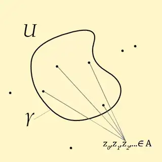
- Residue theorem Let $ U \in \mathbb {C} $ be a simply connected open set (without "holes"), let $ f: U \to \mathbb {C} $ be a meromorphic function. Let $ \gamma: [a, b] \to U $ be a closed and regular curve and $ A = \{z_0, z_1, z_2, \dots \} $ the set of poles of $ f $ contained within the contour of $ \gamma $
$$ \int_{\gamma} f(s)ds =2 \pi i \sum_{z_j \in A}\text{Res}_{z_j}(f) . $$
This theorem tells us that the value of a contour integral, for any contour in the complex plane, corresponds to the sum of the residue of $ f $ at the poles inside the boundary of $ \gamma $.
$ \ $
$ \ $
$$\underline{\text{Sugarcoat it}}$$
Let's start by considering the function
$$ g(N):= \sum_{n=1}^N \frac{1}{n^2}=1+\frac{1}{4}+\frac{1}{9}+\dots+\frac{1}{N^2}. $$
Estimating the limit of $ (2) $ is a famous problem known as the $\underline {\text{Basel problem}}$ which was solved by Euler, who shows that $ g (N) $ converges to $ \pi ^2/6 $ when $ N \to \infty $, or in other words
$$ g(N)=\frac{\pi^2}{6}+o(1) $$
where $ o(1) $ denotes a quantity that goes to zero when $ N \to \infty $. Using the $\underline {\text{integral test}}$ we obtain a more precise result
$$ \sum_{n=N+1}^{\infty}\frac{1}{n^2} \le \int_N^{\infty} \frac{dx}{x^2} =\frac{1}{N} \Rightarrow \sum_{n=1}^{N}\frac{1}{n^2}= \frac{\pi^2}{6}+O(\frac{1}{N}) $$
where $ O (1 / N) $ denotes a quantity that goes to infinity such as $ 1 / N $. Thus we can interpreted $ \pi^ 2/6 $ as the degree zero coefficient of the asymptotic series expansion of $ g (N) $.
$ \ $
All problems arise here, due to the discrete nature of the sum
$$ \sum_{n=1}^N \frac{1}{n^s} \tag{2} $$
which has discontinuities of the first kind (jump) for each positive integer value of $ N $.
Such discontinuities produce various artifacts when trying to expand $ (2) $, generating a polynomial in $ N $, to evaluate its trend. This also occurs in the Basel problem, but in that case the artifacts are included in the $ O (1 / N) $ error, while for $ \Re (s) \le 1$ they become large enough to cause problems. Therefore, for $ \Re (s) <1 $, to set $ (2) $ equal to a constant coefficient plus an error that tends to zero, evidently it is no longer sufficient
It is possible to solve this problem, that is to find the missing terms to the expansion of $ (2) $ when $ \Re (s) <1 $, by intervening on the discontinuous nature of $ (2) $.
We can rewrite $ (2) $ as
$$ \sum_{n=1}^{\infty}\frac{1}{n^s} \mathbb{1}_{[0,1]}\big(\frac{n}{N}\big) $$
in fact when $ 0 \le n \le N $ we have $ \mathbb {1} _ {[0,1]} \big(n / N \big) = 1 $ while for $ n> N $ we will have $ \mathbb {1} _ {[0,1]} \big(n / N \big) = 0 $.
Using a cut off function $ \eta $ it is possible to obtain a "sweeter" version of $ (2) $ while preserving its asymptotic behavior.
$$ \sum_{n=1}^{\infty}\frac{1}{n^s}\eta\big(\frac{n}{N}\big) \tag{3} $$
We will now study $ (3) $ to obtain the expansion of $ (2) $ and show how the coefficient of lower degree is related to $ \zeta (s) $. We could therefore say that for $ N \to \infty $ and $ \Re (s <1) $ it is not possible to equal $ \sum 1 / n^ 2 $ to $ \zeta (s) + O (1 / N) $ which instead is the definition $ (1) $ in the region $ \Re (s> 1) $.
$ \ $
$ \ $
$$\underline{\text{Do the math}}$$
We show how - using Fourier analysis and complex analysis - it is possible to determine the asymptotic behavior of $ \sum \frac {1} {n ^ 2} $ thanks to the meromorphic properties of the $ \zeta $ function.
$ \ $
Let $ s $ be a complex number such that $ \Re (s) <1 $, and $ \eta: \mathbb {R}^{+} \to \mathbb {R} $ a cutoff function that returns one near origin, and consider the expression
$$ \sum_ {n = 1} ^ {\infty} \frac {1} {n ^ s} \eta \big( \frac {n} {N} \big) \tag {3} $$
where $ N $ is a large positive integer. Then let $ A> 0 $ be an integer such that $ \Re (s + A)> 1 $ e $ f_A (x): = e^ {A x} \eta (e ^ x) $, we can rewrite $ (3 ) $ like
$$ N ^ A \sum_ {n = 1} ^ {\infty} \frac {1} {n ^ {s + A}} f_A (\ln (n / N)). $$
Note that $ \eta (x) $ is a Schwartz function whose behavior "dominates" any polynomial, than $ x ^ A \eta (x) $ is still a Schwartz function, so $ f_A (x) \in \mathcal {S} (\mathbb {R}) $. From the Fourier inversion formula, it has representation
$$f_A(x)=\int_{-\infty}^{+\infty}\hat{f}_A(t)e^{-i x t}dt $$
where
$$ \hat{f}_A(t):= \frac{1}{2 \pi}\int_{-\infty}^{+\infty}f_A(x)e^{ixt}dx$$
by definition $ \hat {f}_A (x) $ is also a Schwartz function. We rewrite $ (3) $ as
$$ N^A \sum_{n=1}^{\infty}\frac{1}{n^{s+A}}\int_{-\infty}^{+\infty}\hat{f}_A(t)e^{-i \ln(n/N) t}dt=\int_{-\infty}^{+\infty}\Big(\hat{f}_A(t)N^{A+it} \frac{1}{n^{it}}\sum_{n=1}^{\infty}\frac{1}{n^{s+A}}\Big)dt $$
Since $ \Re (s + A + it)> 1 $ we can use the definition $ \zeta (z) = \sum \frac {1} {n ^ z} $ and write
$$ \sum_{n=1}^{\infty}\frac{1}{n^s}\eta\big(\frac{n}{N}\big)= \int_{-\infty}^{+\infty}\hat{f}_A(t)N^{A+it} \zeta(s+A+it)dt.$$
now we have
$$ \hat{f}_A(x)=\frac{1}{2 \pi}\int_{-\infty}^{+\infty}\eta(e^x)e^{(A+it)x}dx $$
integrating by parts:
$$ \hat{f}_A(x)=\frac{1}{2 \pi}\Big[ \frac{\eta(e^x)e^{(A+it)x}}{A+it} \Big]^{+\infty}_{-\infty}-\frac{1}{2 \pi}\int_{-\infty}^{+\infty}\frac{e^x\eta'(e^x)e^{(A+it)x}}{A+it} $$
having that $ \eta(e^x)(e^x)^c \to 0$ for $ x \to +\infty$ and that $(e^{x})^c\to 0$ for $x \to -\infty$ and $\eta(0)=1$
$$ \hat{f}_A(t)=-\frac{1}{2 \pi(A+it)}\int_{-\infty}^{+\infty}\eta'(e^x)e^{(A+it+1)x}dx=-\frac{1}{2 \pi(A+it)}\int_0^{+\infty}y^{A+it}\eta'(y)dy $$
we define
$$ F(A+it)=\frac{1}{(A+it)}\int_0^{+\infty}y^{A+it}\eta'(y)dy. \tag{4}$$
We have that $ F (A + it) $ is a function entirely of $ A + it $ and furthermore, $ \hat {f} _A (t) \in \mathcal {S} (\mathbb {R}) $, $ \hat {f} _A (t) = - 1 / (2 \pi) F (A + it) $ therefore fixed $ A $, $ F (A + it) $ decreases faster than any polynomial when $ t \to \infty. $
We can rewrite $ (3) $ as
$$ -\frac{1}{2 \pi}\int_{-\infty}^{+\infty}F(A+it)N^{A+it} \zeta(s+A+it)dt $$
set $z=s+A+it$
$$ -\frac{1}{2 \pi i}\int_{s+A-i\infty}^{s+A+i\infty}\zeta(z)F(z-s)N^{z-s} dz. $$
It is known that fixed $ \sigma $, $ \zeta (\ sigma + it) $ has polynomial growth in $ t $ and also that $ \zeta (z) $ has a simple pole at $ z = 1 $ with expansion in that point
$$ \zeta(z)^2=\frac{1}{(z-1)^2}+2 \gamma\frac{1}{z-1}+O(1)\Rightarrow \zeta(z)\sim \frac{1}{z-1} \text{ per } z \to 1 $$
We have from $ (4) $ that $ F (z-s) $ has a simple pole for $ z = s $ so the integrating function $ J (z): = \zeta (z) F (z-s) N ^ {z-s} $ has two simple poles. Let's proceed by calculating the residuals:
$$ \text{Res}_{z=s}[J(z)]=\lim_{z \to s} [J(z) (z-s)]=\zeta(s) \int_0^{+\infty}\eta'(y)dy =\zeta(s)\Big[ \eta(y)\Big]^{+\infty}_0=-\zeta(s) $$
To calculate $ \text{Res}_{z = 1} [J (z)] $ we integrate by parts
$$F(1-s)= \frac{1}{(1-s)}\int_0^{+\infty}y^{1-s}\eta'(y)dy $$
$$F(1-s)= \frac{1}{(1-s)}\Big[\eta(y)y^{1-s} \Big]^{+\infty}_0 -\int_0^{+\infty}y^{-s}\eta(y)dy \tag{5}$$
$ \ Re (s) <1 $ and therefore $ \frac{1}{0^s} = 0 $:
$$F(1-s)= -\int_0^{+\infty}y^{-s}\eta(y)dy$$
the integral of $ y^ {- s} \eta (y) $ is known and is the $\underline{\text{Mellin transform}}$ of $ \eta $, which we will denote by $ \mathcal {M}_{\eta} ( -s) $ and has a non-negative value
$$\text{Res}_{z=1}[J(z)]=\lim_{z \to 1} [J(z)(z-1)]=N^{1-s}F(1-s) =-N^{1-s}\mathcal{M}_{\eta}(-s).$$
From the residue theorem we have that if $ \gamma $ is a contour of the complex plane that contains the poles $ z_1 = 1 $ and $ z_2 = s $ of $ J (z) $, we can evaluate
$$ \int_{\gamma} \zeta(z)F(z-s)N^{z-s}dz=2\pi i \Big(-N^{1-s}\mathcal{M}_{\eta}(-s)-\zeta(s)\Big). $$
Since $ \zeta (\sigma + it) $ has polynomial growth and $ F (\sigma + it) $ decreases faster than any polynomial, $ J (z) $ will go to zero for $ t \to \infty $.
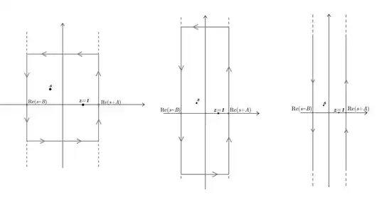
It is therefore possible to choose a $ \gamma $ contour as in the figure, bringing the horizontal paths to infinity, making them negligible. Then applying the residual theorem on $ \gamma $ composed of two lines that include the poles, one from minus infinity to plus infinity and the other from plus infinity to minus infinity. $ \forall B \ | \ \Re (s-B) <\Re (s): $
$$ -\frac{1}{2 \pi i}\Big(\int_{s+A-i\infty}^{s+A+i\infty}J(z) dz+\int_{s-B+i\infty}^{s-B-i\infty}J(z) dz \Big)=\zeta(s)+N^{1-s}\mathcal{M}_{\eta}(-s)$$
$$ -\frac{1}{2 \pi i}\int_{s+A-i\infty}^{s+A+i\infty}J(z) dz=-\frac{1}{2 \pi i}\int_{s-B-i\infty}^{s-B+i\infty}J(z) dz+\zeta(s)+N^{1-s}\mathcal{M}_{\eta}(-s)$$
performing a change of variables
$$ \sum_{n=1}^{\infty}\frac{1}{n^s}\eta\big(\frac{n}{N}\big)=\zeta(s)+N^{1-s}\mathcal{M}_{\eta}(-s)-\frac{N^{-B}}{2 \pi}\int_{-\infty}^{+\infty}\zeta(s-B+i t)F(-B+it)N^{i t}dt \tag{6}$$
by the considerations on the behavior of $ \zeta $ and $ F $, the integral on the right of $ (6) $ converges and has a constant value.
We can finally write for $ \Re (s) <1 $
$$ \sum_{n=1}^{N}\frac{1}{n^s}\eta\big(\frac{n}{N}\big)=\zeta(s)+N^{1-s}\mathcal{M}_{\eta}(-s)+O(N^{-B}) $$
$$ \sum_{n=1}^{N}n=1+2+3+\dots+N=-\frac{1}{12}+N^{2}\mathcal{M}_{\eta}(-1)+O(N^{-B}) $$
We note that for $ \Re (s) <1 $ there is a link between the values obtained by applying algebraic operations $ 1 + 2 + \dots + N $ and the values obtained by analytic continuation $ \zeta (s) $.
We have shown how in this domain it is no longer sufficient to expand the summation - as a polynomial in $ N $ - only to the zero degree term (which can also be negative) but in this case it is necessary to expand up to the second degree term, obtaining the term $ N ^ {2} \mathcal {M}_{\eta} (- 1) $ (which goes to infinity) and therefore the correct asymptotic trend.
$ \ $
By the $\underline{\text{Euler-Maclaurin formula}}$ it is possible to prove that $ \{\forall s \in \mathbb{C}: \Re (s) <1 \} $, the expression
$$ \sum_ {n = 1} ^ {\infty} \frac {1} {n ^ s} \eta \big ( \frac {n} {N} \big) -N ^ {1-s} \mathcal{M}_ {\eta} (- s) $$
converges smoothly for $ N \to \infty $. Moreover from the $\underline {\text{Morera's theorem}}$ it is possible to prove that this limit is complex-analytic therefore we can define $ \zeta $ in $\Re (s) <1$ region as:
$$\zeta(s)=\lim_{N \to \infty} \sum_{n=1}^{\infty}\frac{1}{n^s}\eta\big(\frac{n}{N}\big)-N^{1-s}\mathcal{M}_{\eta}(-s). \tag{7}$$
$ \ $
$ \ $
$$\underline{\text{The Casimir Effect}}$$
In physics, the Casimir effect consists in the attractive force that is exerted between two extended bodies located in the vacuum, for example two parallel plates, due to the presence of the $\underline {\text{zero-point quantum field}}$. This phenomenon is interesting both because the values obtained through the infinite application of arithmetic operations coincide with the values obtained through analytical continuation and because it offers experimental evidence that the vacuum is not really empty.
Classically to calculate the electromagnetic energy contained in an empty box (of dimension $ L \times L \times a $) with conductive walls at $\underline{\text{absolute zero}}$, we have to sum the energy
$$ E=\frac{1}{2} \hbar \omega=\frac{1}{2}\hbar c k$$
(obtained from the quantization of the harmonic oscillator at zero point) for all possible harmonic oscillators, i.e. for all wave numbers $ k $ allowed inside the box:
$$E=2\frac{1}{2}\sum_{x=1}^{\infty}\sum_{y=1}^{\infty}\sum_{n=1}^{\infty}\sqrt{\frac{x^2 \pi^2}{L^2}+\frac{y^2 \pi^2}{L^2}+\frac{n^2 \pi^2}{a^2}} $$
for simplicity we have setted $ \hbar = c = 1 $. Assuming that the $ box $ is one-dimensional with length $ a $ we have:
$$\frac{a}{\hbar c \pi}E=\sum_{n=1}^{\infty}n. \tag{8}$$
From the considerations made in the previous paragraph we can conceptually write $ (8) $ as:
$$\frac{a}{\hbar c \pi}E=-\frac{1}{12}+\infty $$
in this context the term $ \infty $ is exactly canceled from the energy density of the $\underline{\text{ground state}}$ which is outside the box, in the region of space called universe.
From this it could conclude that in this context
$$ \sum_{n=1}^{\infty}n=-\frac{1}{12} $$
but so we will neglect the effect that the universe operates on the box which is what leads to the cancellation of the term $ \infty $.
To make this effect explicit, it is possible to define the $\underline {\text{Casimir energy}}$ in a certain region of space as:
"the difference between the allowed wavelengths, in a region bounded by conductive walls, and the allowed wavelengths if the walls weren't there".
In other words:
$$\frac{a}{\hbar c \pi}E= \sum_{n=1}^{\infty}n-\int_0^{\infty}n\ dn \tag{9}$$
we see that to the right side of $ (9) $ you get $ \infty- \infty $ so we must $\underline{\text{regularize}}$:
$$\frac{a}{\hbar c \pi}E=\lim_{\alpha\to0}\bigg[ \sum_{n=1}^{\infty}n e^{-\alpha n}-\int_0^{\infty}n e^{-\alpha n} dn \bigg]. \tag{10} $$
Regularization is not a mysterious mathematical trick, but it is a physically realistic model that represents the fact that metal is not a good conductor for sufficiently small wavelengths ($ 1 / k $). Also, we performed an exponential regularization, but we would have achieved the same result using any cutoff function. Thus we have that in $ (10) $ the definition of $ \zeta $ expressed in $ (7) $, allowing us to write
$$\frac{a}{\hbar c \pi}E= \zeta(-1)=-\frac{1}{12}.$$ In the three-dimensional case of two parallel plates of unitary area, distant $ a $:
$$\frac{6 a^3}{\hbar c \pi^2}E= \zeta(-3)=\frac{1}{120}.$$
The attraction force will be:
$$ F_c=\frac{d}{d a} E=-\frac{\hbar c \pi^2}{2 a^4}\zeta(-3).$$
Hendrik Casimir predicted this result in 1948. It was only in 1997 that S. Lamoreaux quantitatively measured the force within 5 % of the theoretically predicted value.


