1

I'm trying to understand the actual solution which is computed here (Sec. 4.7 of Ref. (1)), trying to resolve $$ \begin{cases} \displaystyle \frac{\partial u}{\partial \tau} + \frac{\partial q}{\partial x} = 0, \\ u(0,x) = \frac{c_0}{c_{max}} = \begin{cases} 0, \quad \text{if} \quad x \le 0\\ u_0, \quad \text{if} \quad x \in ]0,1[ \\ 1, \quad \text{if} \quad x \ge 1 \end{cases}\\ u(\tau, 0) = 0\\ u(\tau ,h) = 1, \forall\tau > 0 \end{cases} $$ where $q(u) = u(1-u)(1-\beta u)$ with $\frac{1}{2} < \beta < 1$. First, he's trying to connect $0$ to $u_0$ with a shock wave: $$x(\tau) = \sigma(0,u_0)(\tau) = \dfrac{q(u_0)}{u_0}\tau$$ so the solution becomes $ u(t,x) = 0$ if $x <\sigma(0,u_0)\tau$, $u(t,x) = u_0$ if $1 > x >\sigma(0,u_0)\tau$, and $u(t,x) = 1$ if $x \ge 1$. Then he's trying to connect $u_0$ to $1$ by introducing an intermediate state which is $u_1$. How does it change the exact solution? He's only showing the final stationary state at the end.

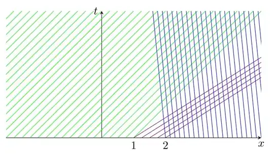
the characteristics:

\begin{center}
\begin{tikzpicture}
\draw[-stealth] (-4,0)--(4,0) node[below]{$x$}; 
\draw[-stealth] (-1,0)--(-1,4) node[left]{$t$}; 
\node[below] at (0,0) {$1$};
\node[below] at (1,0) {$2$};
\clip (-4,0) rectangle (4,4);
\foreach \xi in {-8,-7.75,...,0} \draw[green] (\xi,0) -- (\xi+4,4);
\foreach \xi in {0,0.25,...,1} \draw[violet] (\xi,0) -- (\xi+4*1.575,4);
\foreach \xi in {1,1.15,...,5} \draw[blue] (\xi,0) -- (\xi-4*0.1,4);
\end{tikzpicture}
\end{center}

enter image description here

(1) S Salsa: Partial Differential Equations in Action: From Modelling to Theory, 3rd Ed. Springer, 2016. doi:10.1007/978-3-319-31238-5
EditPiAf
  • 20,898
Rasule
  • 43
  • Thanks, i'm going to look into it.. There is no conditions on $h$ but $u_0$ belongs to $]a,u_f[$ as it is shown in the Fig. 4.30 sec. 4.7 in the PDF where $a = \frac{1-\beta}{\beta}$ and $u_f$ is the inflexion point of the curve q(u), $u_f = \frac{1+\beta}{3 \beta}$ – Rasule Jun 09 '20 at 15:49

2 Answers2

1

As described in the book, there is a rarefaction starting at $x=0$, and a semi-shock starting at $x=1$. The state $u_1$ introduced in the book is where the semi-shock wave transitions from a discontinuity to a smooth rarefaction wave. See this post for a presentation of these waves.

EditPiAf
  • 20,898
  • @rasule If you give me some numerical values for $\beta$, $u_0$, then I can derive the solution on a particular case. – EditPiAf Jun 16 '20 at 09:06
0

This is not a full answer. This is only the general solution of the PDE (Without boundary and initial condition). Hopping that it helps.

$$\frac{\partial u}{\partial \tau} + \frac{\partial q}{\partial x} = 0 \quad\text{with}\quad q(u) = u(1-u)(1-\beta u)$$

I suppose that $\beta=$constant.

$\frac{\partial q}{\partial x}=\big(3\beta u^2-2(\beta+1)u+1\big)\frac{\partial u}{\partial x}$

The PDE explicitly written is :

$$\boxed{\frac{\partial u}{\partial \tau} + \big(3\beta u^2-2(\beta+1)u+1\big)\frac{\partial u}{\partial x} = 0}\tag 1$$

The Charpit-Lagrange system of characteristic ODEs is : $$\frac{d\tau}{1}=\frac{dx}{3\beta u^2-2(\beta+1)u+1}=\frac{du}{0}$$

Finite $\frac{du}{0}$ implies $du=0$. Thus a first characteristic equation is $$u=c_1$$

A second characteristic equation comes from solving $\frac{d\tau}{1}=\frac{dx}{3\beta c_1^2-2(\beta+1)c_1+1}$

$$\big(\beta c_1^2-2(\beta+1)c_1+1\big)\tau-x=c_2$$

The general solution of the PDE expressed on the form of implicit equation $c_2=\Phi(c_1)$ or $c_1=\Psi(c_2)$ is : $$\boxed{u=\Psi\Big(\big(\beta u^2-2(\beta+1)u+1\big)\tau-x\Big)}\tag 2$$ with arbitrary function $\Psi$ (or $\Phi$). The function $\Psi$ (or $\Phi$) has to be determined so that the specified boundary and initial conditions be satisfied.

JJacquelin
  • 66,221
  • 3
  • 37
  • 87
  • So that's where the intermediate state $u_1$ come from? – Rasule Jun 09 '20 at 22:33
  • $u_1$ is an intermediate state between $u_0$ and $1$. It allows us to connect $u_0$ to $u_1$ through an admissible shock and then connect $u_1$ to $1$ with a rarefaction because we cannot connect $u_0$ to $1$ directly, the entropy condition is invalid that way. – Rasule Jun 10 '20 at 08:12
  • This is not the aim of my post. As pointed out at the begining I provide the analytic general solution of the PDE, without any interpretation such as shock which depends on the boundary/initial conditions. For that the arbitray function $\Psi$ or its inverse $\Phi$ has to be determined according to the conditions. – JJacquelin Jun 10 '20 at 08:20
  • My post must not be understood as an answer but as comment (too long to be edited in the comments section). It was given only for information. – JJacquelin Jun 10 '20 at 08:37