5

The first principles of duality in LP state simply that if you have a primal problem of the following form

enter image description here

Then i can write the dual LP automatically as:

enter image description here

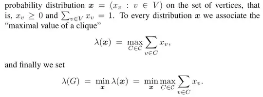
Let $\mathcal{C}$ be the set of cliques in G. Consider an arbitrary

enter image description here

Now how do we write the dual of this bi-level LP? The answer is as follows:

enter image description here

enter image description here

Is there some graph theory trick that I am missing? The dual transformation seems hand-wavy. I am not able to derive it from the first principles as shown above.

EDIT:

I am trying to expound on Misha's answer. There are gaps in my understanding which can hopefully be filled.

In below $z$ is a scalar. $\mathbf{x}\in R^{|V|}$ is a vector. We wish to minimize

$\underset{\mathbf x, z}{\text{min}}\ z$

Now i want to map this to the vanilla model. So $p$ is a vector of $1$ followed by $|V|$ number of zeros, and $x$ is really $z$ concatenated with our probability distribution $\mathbf{x}$. If any symbol is not clear go back to start of the question where i have clearly defined these terms.

Now let me write the constraints one by one as inequalities because i still do not have the hang of equalities in LP, and then I will try to write out the $A$ matrix.

$z - \sum_{v \in C} x_v\ge 0 \text{ for all }C \in \mathcal C$

$\sum_{v \in V} x_v \ge 1$

$-\sum_{v \in V} x_v \ge -1$

And the constraints on the variables are simply:

$z \ge \mathbf 0, \mathbf x \ge \mathbf 0$

Now i want to write down my matrix $A$ and vector $b$ so that from there the dual transformation is straightforward and there is no scope for confusion.

It is clear that $A\in R^{(|\mathcal{C}|+2)\times (|V|+1)|}$ and $b\in R^{(|\mathcal{C}|+2)}$.

Let us first fill $A$ row by row. The first row will be $1$ followed by $|V|$ numbers, some of which will be $-1$ and some will be zero depending on which clique we are considering at that row. Now let us focus on the penultimate row. The first term will be zero followed by $|V|$ numbers of $1$. The last row similarly will have first term as zero followed by $|V|$ numbers of $-1$.

Now we try to write out $b$ which is simply $|V|$ numbers of zeros followed by $1$ and $-1$. Now to perform dual transformation I do need the dual variable to $x$. Please note that $x$ and $\mathbf{x}$ are different things here due to a suboptimal choice of notations in the beginning.

What is the dual variable of $x$? Say it is $w\in R^{|\mathcal{C}|+2}$. So dual problem requires us to maximize as follows:

$\underset{w}{\text{max}}\ b'w$

And $b'w$ is just the difference of the last two terms of $w$ due to structure of $b$. Now there will be $|V|+1$ inequality constraints. But now i am getting confused how to reconcile this with the final answer. Can someone fill the rest? i am trying to make use of this post.

  • 1
    "The dual variable to $x$" doesn't make sense. Variables in the primal correspond to constraints in the dual. You get dual variables by looking at the primal constraints. – Misha Lavrov Mar 18 '20 at 18:30

2 Answers2

4

First, here is a guideline to taking duals in such cases. Often in graph theory problems the matrices are sparse, so we do not want to write out and explicitly take the transpose of the matrix $A$.

Instead, we reason as follows. For each primal constraint, we will get a dual variable; for each primal variable, we will get a dual constraint. To find the coefficients in each dual constraint, we use the following rule, equivalent to taking the transpose of $A$:

If $x_i$ is a primal variable and $u_j$ is a dual variable, the coefficient of $u_j$ in the dual constraint corresponding to $x_i$ is equal to the coefficient of $x_i$ in the primal constraint corresponding to $x_j$.

In particular, $u_j$ appears in the dual constraint corresponding to $x_i$ if and only if $x_i$ appears in the primal constraint corresponding to $u_j$.

I will expand on a few cases of this later on in this answer.


We write $\min_{\mathbf x} \max_{C \in \mathcal C} \sum_{v \in C} x_v$ as the linear program

\begin{aligned} & \underset{\mathbf x, z}{\text{minimize}} && z \\ & \text{subject to} && z \ge \sum_{v \in C} x_v & \text{ for all }C \in \mathcal C \\ &&& \sum_{v \in V} x_v = 1 \\ &&& \mathbf x \ge \mathbf 0, z \text{ unrestricted} \end{aligned} The constraints enforce that $z$ is at least the value of any clique, so it is at least the maximal value of a clique. Since we're minimizing, we will want to set it to the maximal value of a clique, and we will want to pick $\mathbf x$ to make that as small as possible. (We could have made $z$ be a nonnegative variable, but this version will be more similar to the dual.)

Let $\mathbf y \in \mathbb R^{|\mathcal C|}$ be the dual vector associated to the first set of constraints, whose more standard form is $z - \sum_{v \in C} x_v \ge 0$. Let $w$ be the dual variable associated to the constraint $\sum_{v \in V} x_v = 1$.

(I'm also going to be using the idea that equation constraints correspond to unrestricted variables which aren't required to be nonnegative. This isn't quite vanilla, so let me know if you'd like me to elaborate. Briefly, we can write an unrestricted variable $z$ as the difference $z^+ - z^-$ where $z^+, z^- \ge 0$, and we can write an equation as two inequalities.)

Now we write down the dual, taken in the standard way:

\begin{aligned} & \underset{\mathbf y, w}{\text{maximize}} && w \\ & \text{subject to} && w - \sum_{C \ni v} y_C \le 0 & \text{for all } v \in V \\ &&& \sum_{C \in \mathcal C} y_C = 1 \\ &&& \mathbf y \ge \mathbf 0, w \text{ unrestricted} \end{aligned} To see the details of where the constraints come from:

  • $y_C$ appears in the constraint for vertex $v$ if and only if $x_v$ appears in the constraint for clique $C$. The coefficients of $x_v$ in these primal constraints are all $-1$ (if they're not $0$), so the coefficients of $y_C$ are all $-1$ as well (if they're not $0$).
  • $w$ appears in the constraint for every vertex with a coefficient of $1$, because every single $x_v$ appears in the constraint $\sum_v x_v = 1$ with a coefficient of $1$.
  • The final constraint corresponds to primal variable $z$. Since $z$ appears in the constraint for every clique with a coefficient of $1$, every $y_C$ appears in the final constraint, also with a coefficient of $1$.

In the dual, $w$ is forced to be the min of several terms. It is less than $\sum_{C \ni v} y_C$ for each vertex $v$, so it is less than the minimum of those sums; since we're maximizing, we want to set it equal to the minimum of those sums. This is now exactly the problem we're writing in shorthand as $$ \max_{\mathbf y} \min_{v \in V} \sum_{C \ni v} y_c $$ where the maximum is over all distributions $\mathbf y$.

Misha Lavrov
  • 142,276
  • Also why did you choose z to be unrestricted? Isn't z supposed to be greater or equal to sum of probability values? In my version I have taken z to be nonnegative to make the LP standard? – user_1_1_1 Mar 18 '20 at 12:00
  • refer to my edit above please. – user_1_1_1 Mar 18 '20 at 12:35
  • We could choose to make $z$ nonnegative, because it's greater than or equal to the sum of probability values. It's cleaner to make it unrestricted. If we made $z$ nonnegative, we'd get $\sum_C y_C \le 1$ in the dual program, but then we can argue that an optimal solution still has $\sum_C y_C = 1$. – Misha Lavrov Mar 18 '20 at 18:28
  • I've added more details about how to find the coefficients in the constraints without writing out the matrix $A$. – Misha Lavrov Mar 18 '20 at 18:28
  • Thx for clearing all my doubts except one. If we made z nonnegative, how would you argue that an optimal solution holds only at the equality? By simply stating that since we want to maximize w, so more the value of $\sum_C y_C $ the better, right? – user_1_1_1 Mar 19 '20 at 11:06
  • 1
    That's the idea. To put it more formally, if $\sum_C y_C = s < 1$, you could replace $\mathbf y$ and $w$ by $\frac1s \mathbf y$ and $\frac ws$ respectively, which increase the value of the objective function but still satisfies all the constraints. – Misha Lavrov Mar 19 '20 at 18:15
1

There's another way to see the conclusion of this problem without explicitly writing down an LP dual; that's to use the theory of zero-sum games.

Consider a game between players named Vertex and Clique. To play, Vertex picks a vertex $v \in V$, while Clique simultaneously picks a clique $C \in \mathcal C$. Then, if $v \in C$, Vertex gives a dollar to Clique. If $v \notin C$, no money is exchanged.

If Vertex is playing a mixed strategy $\boldsymbol x$ which picks vertex $v$ with probability $x_v$, then $\max_{C \in \mathcal C} \sum_{v \in C} x_v$ is the maximum expected amount Clique can earn in response to $\boldsymbol x$. Thus, Vertex's minimax strategy loses precisely $$\lambda(G) = \min_{\boldsymbol x}\max_{C \in \mathcal C} \sum_{v \in C} x_v$$ dollars each time the game is played, in expectation (assuming best play by Clique).

Similarly, if Clique is playing a mixed strategy $\boldsymbol y$ which picks clique $C$ with probability $y_C$, then $\min_{v \in V} \sum_{C \ni v} y_C$ is the minimum expected amount Vertex can lose in response to $\boldsymbol y$. Thus, Clique's maximin strategy earns precisely $$\max_{\boldsymbol y} \min_{v \in V} \sum_{C \ni v} y_C$$ dollars each time the game is played, in expectation (assuming best play by Vertex).

The minimax theorem for zero-sum games says that Vertex's minimax strategy has the same value (that is, expected amount Clique gets from Vertex) as Clique's maximin strategy, which is precisely the equation we wanted.

(This is essentially the same idea as LP duality, in heavy disguise.)

Misha Lavrov
  • 142,276