Limiting distribution of $\frac1n \sum_{k=1}^{n}|S_{k-1}|(X_k^2 - 1)$ where $X_k$ are i.i.d standard normal

Question

Let $(X_n)$ be a sequence of i.i.d $\mathcal N(0,1)$ random variables. Define $S_0=0$ and $S_n=\sum_{k=1}^n X_k$ for $n\geq 1$. Find the limiting distribution of $$\frac1n \sum_{k=1}^{n}|S_{k-1}|(X_k^2 - 1)$$

This problem is from Shiryaev's Problems in Probability, in the chapter on the Central Limit Theorem. It was asked on this site in 2014, but remains unanswered. I posted it yesterday on Cross Validated, and I think it's worth to cross-post it here as well.

Since $S_{k-1}$ and $X_k$ are independent, $E(|S_{k-1}|(X_k^2 - 1))=0$ and $$V(|S_{k-1}|(X_k^2 - 1)) = E(S_{k-1}^2(X_k^2 - 1)^2)= E(S_{k-1}^2)E((X_k^2 - 1)^2) =2(k-1)$$

Note that the $|S_{k-1}|(X_k^2 - 1)$ are clearly not independent. However, as observed by Clement C. in the comments, they are uncorrelated since for $j>k$ $$\begin{aligned}Cov(|S_{k-1}|(X_k^2 - 1), |S_{j-1}|(X_j^2 - 1)) &= E(|S_{k-1}|(X_k^2 - 1)|S_{j-1}|)E(X_j^2 - 1)\\ &=0 \end{aligned}$$

Hence $\displaystyle V(\frac1n \sum_{k=1}^{n}|S_{k-1}|(X_k^2 - 1)) = \frac 1{n^2}\sum_{k=1}^{n} 2(k-1) = \frac{n-1}n$ and the variance converges to $1$.

I have run simulations to get a feel of the answer

import numpy as np
import scipy as sc
import scipy.stats as stats
import matplotlib.pyplot as plt

n = 30000 #summation index
m = 10000 #number of samples

X = np.random.normal(size=(m,n))
sums = np.cumsum(X, axis=1)
sums = np.delete(sums, -1, 1)
prods = np.delete(X**2-1, 0, 1)*np.abs(sums)
samples = 1/n*np.sum(prods, axis=1)

plt.hist(samples, bins=100, density=True)
plt.show()

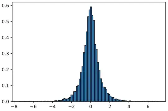
Below is a histogram of $10.000$ samples ($n=30.000$). The variance from the generated samples is $0.9891$ (this complies with the computations above). If the limiting distribution was $\mathcal N(0,\sigma^2)$, then $\sigma=1$. However the histogram peaks at around $0.6$, while the max of the density of $\mathcal N(0,1)$ is $\frac 1{\sqrt{2 \pi}}\approx 0.4$. Thus simulations suggest that the limiting distribution is not Gaussian.

It might help to write $|S_{k-1}| = (2\cdot 1_{S_{k-1}\geq 0} -1)S_{k-1}$.

It might also be helpful to note that if $Z_n=\frac1n \sum_{k=1}^{n}|S_{k-1}|(X_k^2 - 1)$, conditioning on $(X_1,\ldots,X_{n-1})$ yields $$E(e^{itnZ_n}) = E\left(e^{it(n-1)Z_{n-1}} \frac{e^{-it|S_{n-1}|}}{\sqrt{1-2it|S_{n-1}|}}\right)$$

Answer 1

Let $(X_n)_{n\geq 1}$ be a sequence of i.i.d. standard normal variables. Let $(S_n)_{n\geq 0}$ and $(T_n)_{n\geq 0}$ be given by

$$ S_n = \sum_{i=1}^{n} X_i \qquad\text{and}\qquad T_n = \sum_{i=1}^{n} (X_i^2 - 1). $$

We will also fix a partition $\Pi = \{0 = t_0 < t_1 < \cdots < t_k = 1\}$ of $[0, 1]$. Then define

$$ \begin{gathered} Y_n = \frac{1}{n}\sum_{i=1}^{n} | S_{i-1} | (X_i^2-1), \\ Y_{\Pi,n} = \frac{1}{n} \sum_{j=1}^{k} |S_{\lfloor nt_{j-1}\rfloor}| (T_{\lfloor nt_j\rfloor} - T_{\lfloor nt_{j-1} \rfloor}). \end{gathered}$$

Ingredient 1. If $\varphi_{X}(\xi) = \mathbb{E}[\exp(i\xi X)]$ denotes the characteristic function of the random variable $X$, then the inequality $|e^{ix} - e^{iy}| \leq |x - y|$ followed by Jensen's inequality gives

\begin{align*} \big| \varphi_{Y_n}(\xi) - \varphi_{Y_{\Pi,n}}(\xi) \big|^2 &\leq \xi^2 \mathbb{E}\big[ (Y_n - Y_{\Pi,n})^2 \big] \\ &= \frac{\xi^2}{n^2}\sum_{j=1}^{k} \sum_{i \in (nt_{j-1}, nt_j]} 2 \mathbb{E} \big[ \big( | S_{\lfloor n t_{j-1} \rfloor} | - | S_{i-1} | \big)^2 \big]. \end{align*}

From the reverse triangle inequality, the inner expectation is bounded by

\begin{align*} 2 \mathbb{E} \big[ \big( | S_{\lfloor n t_{j-1} \rfloor} | - | S_{i-1} | \big)^2 \big] \leq 2 \mathbb{E} \big[ \big( S_{i-1} - S_{\lfloor n t_{j-1} \rfloor} \big)^2 \big] = 2(i-1-\lfloor nt_{j-1} \rfloor), \end{align*}

and summing this bound over all $i \in (nt_{j-1}, nt_j]$ yields

$$ \big| \varphi_{Y_n}(\xi) - \varphi_{Y_{\Pi,n}}(\xi) \big|^2 \leq \frac{\xi^2}{n^2} \sum_{j=1}^{k} (\lfloor n t_j \rfloor - \lfloor n t_{j-1} \rfloor)^2 \xrightarrow[n\to\infty]{} \xi^2 \sum_{j=1}^{k} (t_j - t_{j-1})^2. \tag{1} $$

Ingredient 2. From the Multivariate CLT, we know that

$$ \Bigg( \frac{S_{\lfloor nt_j\rfloor} - S_{\lfloor nt_{j-1}\rfloor}}{\sqrt{n}}, \frac{T_{\lfloor nt_j\rfloor} - T_{\lfloor nt_{j-1}\rfloor}}{\sqrt{n}} : 1 \leq j \leq k \Bigg) \xrightarrow[n\to\infty]{\text{law}} ( W_{t_j} - W_{t_{j-1}}, N_j : 1 \leq j \leq k ), $$

where $W$ is the standard Brownian motion, $N_j \sim \mathcal{N}(0, 2(t_j - t_{j-1}))$ for each $1 \leq j \leq k$, and all of $W, N_1, \cdots, N_k$ are independent. By the continuous mapping theorem, this shows that

$$ Y_{\Pi,n} \xrightarrow[n\to\infty]{\text{law}} \sum_{j=1}^{k} W_{t_{j-1}} N_j. $$

Moreover, conditioned on $W$, the right-hand side has normal distribution with mean zero and variance $2\sum_{j=1}^{k} W_{t_{j-1}}^2 (t_j - t_{j-1}) $, and so,

$$ \lim_{n\to\infty} \varphi_{Y_{\Pi,n}}(\xi) = \mathbb{E}\left[ \exp\bigg( -\xi^2 \sum_{j=1}^{k} W_{t_{j-1}}^2 (t_j - t_{j-1}) \bigg) \right]. \tag{2} $$

Ingredient 3. Again let $W$ be the standard Brownian motion. Since the sample path $t \mapsto W_t$ is a.s.-continuous, we know that

$$ \sum_{j=1}^{k} W_{t_{j-1}}^2 (t_j - t_{j-1}) \longrightarrow \int_{0}^{1} W_t^2 \, \mathrm{d}t $$

almost surely along any sequence of partitions $(\Pi_k)_{k\geq 1}$ such that $\|\Pi_k\| \to 0$. So, by the bounded convergence theorem,

$$ \mathbb{E}\left[ \exp\bigg( -\xi^2 \sum_{j=1}^{k} W_{t_{j-1}}^2 (t_j - t_{j-1}) \bigg) \right] \longrightarrow \mathbb{E}\left[ \exp\bigg( -\xi^2 \int_{0}^{1} W_t^2 \, \mathrm{d}t \bigg) \right] \tag{3} $$

as $k\to\infty$ along $(\Pi_k)_{k\geq 1}$.

Conclusion. Combining $\text{(1)–(3)}$ and letting $\|\Pi\| \to 0$ proves that

$$ \lim_{n\to\infty} \varphi_{Y_n}(\xi) = \mathbb{E}\left[ \exp\bigg( -\xi^2 \int_{0}^{1} W^2_t \, \mathrm{d}t \bigg) \right], $$

and therefore $Y_n$ converges in distribution to $\mathcal{N}\big( 0, 2\int_{0}^{1} W_t^2 \, \mathrm{d}t \big)$ as desired.

Answer 2

An idea is to use the following result in Martingale limit theory and its applications by Hall and Heyde (Theorem 3.2):

Let $(X_{n,i},\mathcal F_{n,i})_{1\leqslant i\leqslant k_n,n\geqslant 1 }$ by a martingale differences array where $X_{n,i}\in L^2$ and $\mathcal F_{n,i-1}\subset \mathcal F_{n,i}$ for all $n$ and $i$. Suppose that there exists a random variable $\eta^2$ which is a.s. finite and such that

1. $\max_{1\leq i\leq k_n} \left\lvert X_{n,i}\right\rvert\to 0$ in probability;
2. $\sup_{n\geqslant 1}\mathbb E\left[\max_{1\leq i\leq k_n}X_{n,i}^2\right]$ is finite.
3. $\sum_{i=1}^{k_n}X_{n,i}^2\to \eta^2$ in probability;

Then $\sum_{i=1}^{k_n}X_{n,i}\to Z$ in distribution, where $Z=\eta N$, with $N$ standard normal and independent of $\eta$.

However, unfortunately, I am not sum whether this works because here. The sum of the conditional variances converges in law and not in probability.

We will use this result with $\mathcal F_{n,i}=\sigma(X_j,1\leq j\leq n)$, $k_n=n$ and $X_{n,i}=\frac 1n\left\lvert S_{i-1}\right\rvert (X_i^2-1)$.

1. For a fixed $\varepsilon$, $$\mathbb P\left(\max_{1\leq i\leq n} \frac 1n\left\lvert S_{i-1}\right\rvert \left\lvert X_i^2-1\right\rvert>\varepsilon \right) \leqslant \sum_{i=2}^n \mathbb P\left( \left\lvert S_{i-1}\right\rvert \left\lvert X_i^2-1\right\rvert>n\varepsilon \right).$$ Using the independence between $S_{i-1}$ and $X_i$ and the fact that $S_{i-1}$ has a normal distribution with variance $i-1$, we get that
   $$\mathbb P\left( \left\lvert S_{i-1}\right\rvert \left\lvert X_i^2-1\right\rvert>n\varepsilon \right)=\mathbb P\left( \sqrt{i-1}\left\lvert X_1 \right\rvert \left\lvert X_2^2-1\right\rvert>n\varepsilon \right)\leq \mathbb P\left( \left\lvert X_1 \right\rvert \left\lvert X_2^2-1\right\rvert>n^{1/2}\varepsilon \right)$$ and we conclude that 1. holds by the integrability of $\left\lvert X_1 \right\rvert \left\lvert X_2^2-1\right\rvert$.

2. It follows from the fact that $$\mathbb E[X_{n,i}^2]=\frac 1{n^2}(i-1)\mathbb E\left[(X_1^2-1)^2\right]$$ hence we even have finiteness of $\sup_{n\geqslant 1}\mathbb E\left[\sum_{1\leq i\leq k_n}X_{n,i}^2\right].$

3. For the third condition, it would be better to deal with conditional variances. Let $$ \delta_n:= \frac 1{n^2}\sum_{i=2}^n\left( S_{i-1}^2 (X_i^2-1)^2-\mathbb E\left[S_{i-1}^2 (X_i^2-1)^2\mid \mathcal F_{n,i-1}\right]\right). $$ Then $\delta_n$ is a sum of martingale differences and we can check that $\mathbb E\left[\delta_n^2\right]\to 0$. Therefore, we have to look at the limit in probability of $$ A_n:=\frac 1{n^2}\sum_{i=1}^nS_{i}^2= \frac 1n \sum_{i=1}^n W_{i/n}^2, $$ where the equality takes place in distribution and $(W_t)_{t\in [0,1]}$ is a standard Brownian motion. The latter quantity converges in probability to $\int_0^1 W(t)^2dt=:\eta^2$. But there is no convergence in probability. Indeed, $$A_{2n}-A_n= \frac 1{n^2}\sum_{i=1}^nS_i^2-\frac{3}{4n^2}\sum_{i=n+1}^{2n}S_i^2\overset{\mbox{law}}{=}\frac 1n\sum_{i=1}^nW_{i/(2n)}^2-\frac{3}{4n}\sum_{i=n+1}^{2n}W_{i/(2n)}^2.$$