Coordinate-free proof of $\operatorname{Tr}(AB)=\operatorname{Tr}(BA)$?

Question

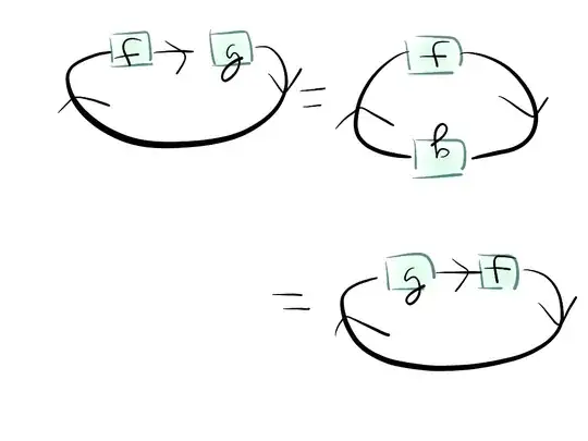
I am searching for a short coordinate-free proof of $\operatorname{Tr}(AB)=\operatorname{Tr}(BA)$ for linear operators $A$, $B$ between finite dimensional vector spaces of the same dimension.

The usual proof is to represent the operators as matrices and then use matrix multiplication. I want a coordinate-free proof. That is, one that does not make reference to an explicit matrix representation of the operator. I define trace as the sum of the eigenvalues of an operator.

Ideally, the proof the should be shorter and require fewer preliminary lemmas than the one given in this blog post.

I would be especially interested in a proof that generalizes to the trace class of operators on a Hilbert space.

Answer 1

$\newcommand{\tr}{\operatorname{tr}}$Here is an exterior algebra approach. Let $V$ be an $n$-dimensional vector space and let $\tau$ be a linear operator on $V$. The alternating multilinear map $$ (v_1,\dots,v_n) \mapsto \sum_{k=1}^n v_1 \wedge\cdots\wedge \tau v_k \wedge\cdots\wedge v_n $$ induces a unique linear operator $\psi: \bigwedge^n V \to \bigwedge^n V$. The trace $\tr(\tau)$ is defined as the unique number satisfying $\psi = \tr(\tau)\iota$, where $\iota$ is the identity. (This is possible because $\bigwedge^n V$ is one-dimensional.)

Let $\sigma$ be another linear operator. We compute \begin{align} (\tr\sigma)(\tr\tau) v_1 \wedge\cdots\wedge v_n &= \sum_{k=1}^n (\tr\sigma) v_1 \wedge\cdots\wedge \tau v_k \wedge\cdots\wedge v_n \\ &= \sum_{k=1}^n v_1 \wedge\cdots\wedge \sigma \tau v_k \wedge\cdots\wedge v_n \\ & \qquad + \sum_{k=1}^n \sum_{j \ne k} v_1 \wedge\cdots\wedge \sigma v_j \wedge \cdots \wedge \tau v_k \wedge\cdots\wedge v_n. \end{align}

Notice that the last sum is symmetric in $\sigma$ and $\tau$, and so is $(\tr\sigma)(\tr\tau) v_1 \wedge\cdots\wedge v_n$. Therefore $$ \sum_{k=1}^n v_1 \wedge\cdots\wedge \sigma \tau v_k \wedge\cdots\wedge v_n = \sum_{k=1}^n v_1 \wedge\cdots\wedge \tau \sigma v_k \wedge\cdots\wedge v_n, $$ i.e. $\tr(\sigma\tau)=\tr(\tau\sigma)$.

---

EDIT: To see that the trace is the sum of all eigenvalues, plug in your eigenvectors in the multilinear map defined at the beginning.

Answer 2

The proof in Martin Brandenburg's answer may look scary but it is secretly about moving beads around on a string. You can see all of the relevant pictures in this blog post and in this blog post. The proof using pictures is the following:

In the first step $g$ gets slid down on the right and in the second step $g$ gets slid up on the left.

You can also find several proofs of the stronger result that $AB$ and $BA$ have the same characteristic polynomial in this blog post.

Answer 3

The trace of an endomorphism $f : X \to X$ of a dualizable object $X$ in a monoidal category is the composition $1 \xrightarrow{\eta} X \otimes X^* \xrightarrow{f \otimes \mathrm{id}} X \otimes X^* \cong X^* \otimes X \xrightarrow{\epsilon} 1$. This coincides with the usual definition in the category of vector spaces. There is a more general categorical notion of trace, which then also applies to Hilbert spaces. Under suitable assumptions the formula $\mathrm{tr}(f \circ g)=\mathrm{tr}(g \circ f)$ holds. For more details, see the paper Traces in monoidal categories by Stolz and Teichner.

Answer 4

Hint Compare the characteristic polynomials of $AB$ and $BA$.

The determinant (whence characteristic polynomials) admits basis-free definitions.

We have $$ \left(\matrix{I&A\\B&tI}\right)\left(\matrix{tI&-A\\0&I}\right)=\left(\matrix{tI&0\\*&tI-BA}\right) $$ and $$ \left(\matrix{I&A\\B&tI}\right)\left(\matrix{tI&0\\-B&I}\right)=\left(\matrix{tI-AB&*\\0&tI}\right). $$ Applying the determinant to these equations yields $$ t^m\det(tI-AB)=t^n\det(tI-BA). $$

Now over an algebraically closed field, we can define the eigenvalues of a linear operator as the zeros of its characteristic polynomial counted with multiplicities. The trace, which you defined as the sum of the latter, is $-1$ times the coefficient of degree $k-1$. So the formula above proves in particular that $\mathrm{tr}(AB)=\mathrm{tr}(BA)$.

Note I don't know how to prove without refering to any basis that the characteristic polynomial is actually a polynomial of degree $k$ with leading coefficient $1$. So I'm afraid this is a bit circular. Anyway, I don't think this is a very convenient way of defining the trace. For a viewpoint which is more useful when seeking infinite-dimensional generalizations, that other answer is probably more useful than what I just wrote above.

Answer 5

The following is a simple combinatorial interpretation of this identity. Not exactly what you asked for, but still fun and relevant.

Suppose we have two sets $S,T$ with functions $g: S \to T$ and $f : T \to S$. Then $f\circ g : S \to S$ and $g\circ f: T \to T$ are endo-functions of $S$ and $T$ respectively. Now consider $\text{Fix}(f\circ g) \subseteq S$, the set of fixed points of $f\circ g$. It is easy to verify that

$$f|_{\text{Fix} (fg)}: \text{Fix} (fg) \to \text{Fix} (gf)$$

is a bijection, with inverse $g|_{\text{Fix} (gf)}$. Therefore, if $S,T$ are finite,

$$|\text{Fix} (fg)| = |\text{Fix} (gf)|.$$

But if $S,T$ are finite, we can represent $f$ as a $|S| \times |T|$ matrix and $g$ as a $|T| \times |S|$ matrix, each with $0$'s and $1$'s. (This matrix depends on an ordering of each set.) Then their products in either order represent the endo-functions $fg$ and $gf$. But it is obvious that for the matrix of an endo-function $h$, $|\text{Fix }h| = \text{Tr}(h)$ (irrespective of the order chosen). Thus, by the above, we $\text{Tr}(fg)=\text{Tr}(gf)$.

Answer 6

In addition to the variety of useful perspectives already given: much as in Martin Brandenberg's answer, but less abstractly, while still coordinate-free... the map $V\otimes V^*\rightarrow \mathrm{End}(V)$ induced from the bilinear map $v\times \lambda\rightarrow (w\rightarrow \lambda(w)\cdot v)$ is a surjection for finite-dimensional vector spaces $V$. Composition is $(v\otimes \lambda)\circ (w\otimes\mu)=\lambda(w)\cdot v\otimes \mu$. Trace is the map induced by $v\times \lambda\rightarrow \lambda(v)$. The fact that $\mathrm{trace}(AB)=\mathrm{trace}(BA)$, $$ \mathrm{trace}((v\otimes \lambda)\circ (w\otimes \mu)) \;=\; \mathrm{trace}(\lambda(w)\cdot v\otimes \mu) \;=\; \lambda(w)\cdot \mu(v) $$ which is obviously symmetric. For the analogue in Hilbert spaces, first use the coordinate-independent characterization of trace-class as composition of two Hilbert-Schmidt operators. The latter are limits of finite-rank operators in the Hilbert-Schmidt norm $|T|_{hs}^2=\mathrm{trace}(T^*T)$, where $T^*$ is adjoint. The comparison of traces of $AB$ and $BA$ is preserved in the limit.

Answer 7

Here is a proof that shows more:

If $A$ and $B$ are such that both $AB$ and $BA$ are square matrices then $AB$ and $BA$ have the same non-zero eigenvalues.

Proof: Let $\lambda \ne 0$ be an eigenvalue and $e$ the eigenvector of $B$. Since $AB~e= \lambda e$ we have $B e \ne 0$. Hence $$ (BA) (Be) = B (AB) e = B (\lambda e) = \lambda (Be) $$ Hence $\lambda $ is also an eigenvalue of $BA$ (with eigenvector $Be$). One can extend this argument to repeated eigenvalues with generalized eigenvectors.

Since trace = sum of eigenvalues, the result follows.

Answer 8

By spectral theorem (which is coordinate-free) unitaries span the whole algebra of operators. So it suffices to prove $\mathrm{Tr}(U_1 U_2) = \mathrm{Tr}(U_2 U_1)$ for unitaries $U_1, U_2$ and this is obvious, since $U_2 U_1 = U_2 (U_1 U_2) U_2^{-1}$ and similar operators certainly have the same eigenvalues (with equal multiplicities).

Answer 9

There always exists an orthonormal bais $|n \rangle$ in our vector space, so you can expand the identity with $1 = \sum_n |n \rangle\langle n| $

\[tr(AB) = \sum_n \langle n|AB |n \rangle =\sum_{m,n} \langle n|A|m \rangle \langle m|B |n \rangle \]

and then you can run it backwards:

\[ = \sum_{m,n} \langle m|B |n \rangle\langle n|A|m \rangle = \sum_{m} \langle m|B A|m \rangle = tr (BA)\]

---

Here I'm using Dirac bra-ket notation from physics.

The vectors $|n\rangle= v_n, n = 1, \dots, n$ form a basis of your vector space. Then $\langle n |$ is like a dual-vector.

The identity matrix has is the sum of projection operators.

\[ 1 = \sum |n\rangle \langle n | = \left[\begin{array}{cccc}1 & 0 &\dots & 0 \\\\ 0 & 1 & \dots & 0 \\\\ \vdots & \vdots & \ddots & \vdots \\\\ 0 & 0 & \dots & 1\end{array} \right] \]

The trace is the sum over diagonals, no matter which basis vectors we choose.

\[tr(AB) = \sum_n \langle n|AB |n \rangle \]

Answer 10

Let there be a vector derivative operator $\partial_a$ that differentiates with respect to a vector $a$. That is, $\partial_a = e^1 \partial_{a^1} + e^2 \partial_{a^2} + \ldots$, where $a = a^1 e_1 + a^2 e_2 + \ldots$ and $e_1, e_2, \ldots$ are basis vectors. Though $\partial_a$ has been defined with respect to some specific frame, it is nevertheless a coordinate-free object.

The trace of a linear operator $\underline A$ can be represented as $\partial_a \cdot \underline A(a)$. Call this quantity $A$, without an underline.

The trace of $\underline A \underline B$ can then be found using the chain rule, as well as the definition of the transpose, $\overline B(a) \cdot b = \underline B(b) \cdot a$. We also use the result $\partial_a \cdot X(a) = \partial_b \cdot [(b \cdot \partial_a)X(a)]$. This makes it possible to apply the chain rule.

$$\begin{align*}\partial_a \cdot \underline A \underline B(a) &= \partial_b \cdot [(b \cdot \partial_a )(\underline A \circ \underline B)(a)] \\ &= \partial_b \cdot [(b \cdot \partial_a \underline B[a]) \cdot \partial_a \underline A(a)] \\ &= \partial_b \cdot [\underline B(b) \cdot \partial_a \underline A(a)] \\ &= \partial_b \cdot [b \cdot \overline B(\partial_a) \underline A(a)] \\ &= \overline B(\partial_a) \cdot \underline A(a) \\ &= \partial_a \cdot \underline B \underline A(a)\end{align*}$$

All one needs to be able to prove this is a good set of vector derivative identities, a little linear algebra, and a coordinate-free notion of the chain rule.