Empirical error proof Runge-Kutta algorithm when not knowing exact solution

Question

I'm implementing a RK solver for calculating the solution to the Lorenz system:

\begin{equation} \begin{cases} x'(t) = \sigma(y-x) \\ y'(t) = rx-y-z \\ z'(t) = xy-bz \end{cases} \end{equation}

The implemented RK method is of order 3 with some random Butcher tableau (but satisfies the conditions neccesary for it to have global error of order $\mathcal{O}(h^k)$, for $k$ the order of the method and local truncation error of $\mathcal{O}(h^{k+1})$).

One of the questions I'm being asked is to prove empirically that my implemented RK achieves these orders of error.

My first attempt was to estimate the local error ($\delta_L$) as: $$\delta_L(t_n) = x_n(t_n)-x_n(t_n-1)$$ Where $x_n$ is the numerical solution of $x$ and $t_n$ is the time step. Following this approach, I get a very oscillatory error, ranging from $-2.5$ to 2.5 with mean $0.0012$, suggesting that the way I calculate the error must not be appropiate.

So you mean $\delta_L(n) = x_n - x_{n-1}$? if this is the way you are calculating it, then you are basically getting $\sim\dot{x}(t_n)\delta t = \sigma(y_n - x_n)\delta t$ — caverac, Jan 01 '19 at 11:00
That's why the solution oscillates. To test the accuracy of your integrator, you should use a system for which you know the solution and calculate the difference between what you expect and what you calculate — caverac, Jan 01 '19 at 11:06
For instance, you can use the harmonic oscillator $\dot x=y$, $\dot y=-x$ with solution $x(t)=\sin t$, $y(t)=\cos t$. // Why use a random method and not some nice one like the order 3 method found by Heun in 1900 and named by Kutta as Heun's method one year later? — Lutz Lehmann, Jan 01 '19 at 18:30
@LutzL You are absolutely right, and you guys made me realize that maybe I interpreted the question in a wrong way. First, I'm going to just test my algorithm with a system I know the exact solution to and check that the order of error is achieved. Finally, I wanted to remark that Butcher's table coefficients are calculated through my personal ID number. This is a way to prevent people from copy pasting basically, which is very common in Spain. Thanks for your time! — Jorge, Jan 02 '19 at 00:47

Lutz Lehmann · Answer 1 · 2019-09-16T07:56:36.160

A classical 3rd order method

As an example method use the Heun 3rd order method (Karl Heun 1900) \begin{array}{l|lll} 0&\\ \frac13&\frac13\\ \frac23&0&\frac23\\ \hline &\frac14&0&\frac34 \end{array}

with the code

def Heun3integrate(f, t, y0):
    dim = len(y0);
    y = np.zeros([len(t),dim]);
    y[0,:] = y0;
    k = np.zeros([4,dim]);
    for i in range(0,len(t)-1):
        h = t[i+1]-t[i];
        k[0,:] = f(t[i], y[i]);
        k[1,:] = f(t[i]+h/3, y[i]+h/3*k[0]);
        k[2,:] = f(t[i]+2*h/3, y[i]+2*h/3*k[1]);
        y[i+1,:] = y[i]+h/4*(k[0]+3*k[2]);
    return y

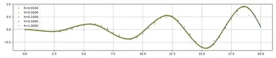
Test using the method of manufactured solutions (MMS)

To verify the correctness of the implementation one can use the idea of manufactured solutions to generate a test problem $F[y]=F[p]$ with known exact solution $p$, like in $F[y]=y''+sin(y)$, $p=\sin t$, that is, $$ y''+\sin(y) = -\sin(t)+\sin(\sin(t)), ~~ y(0)=p(0)=\sin(0)=0,~ y'(0)=p'(0)=\cos(0)=1 $$

def mms_ode(t,y): return np.array([ y[1], sin(sin(t))-sin(t)-sin(y[0]) ])

to get a plot for the error profiles in $y$. To compare a variety of step sizes, scale the error by $h^{-3}$ so that the plot in principle shows the leading error coefficients of the global error over time. If the single graphs appear to be converging to a single function, this confirms the third order. If the third order assumption were wrong one would expect wildly differing scales due to the wrong exponent of $h$.

for h in [1.0, 0.5, 0.1, 0.05, 0.01][::-1]:
    t = np.arange(0,20,h);
    y = Heun3integrate(mms_ode,t,[0,1])
    plt.plot(t, (y[:,0]-np.sin(t))/h**3, 'o', ms=2, label = "h=%.4f"%h);
plt.grid(); plt.legend(); plt.show()

Et voi-la

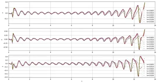
Test on the Lorenz system via step doubling

There is no exact solution of the Lorenz system to use as reference. To still get an error estimate, compute a second solution with double the step size and use Richardson extrapolation to compute the error estimate.

t1 = np.arange(0,tf,h);
u1 = Heun3integrate(Lorenz,t1,[1,1,1])
t2 = t1[::2]
u2 = Heun3integrate(Lorenz,t2,[1,1,1])
err = (u2[:,:]-u1[::2,:])/7

err is the error for the step size h, even if it uses the time scale t2. Then as before plot the error profiles, now scaled by $(h/h_0)^{-3}$ so that the scale is exact for the largest step size, and by $(t+h)^{-1}$ to account for the continuing error accumulation. The plots again show convergence to the same profile curve. The time interval however is rather small for the Lorenz attractor. To get the typical picture one needs at least an integration interval of length $50$. That however will lead to rapidly increasing amplitude of the error profile curve and larger influence of the nonlinear, chaotic nature of the system to the computed trajectories, making them diverge for the different step sizes.

I really like this approach and I will probably implement it for this project! Thanks for elaborating your answer !! — Jorge, Jan 02 '19 at 00:49

Empirical error proof Runge-Kutta algorithm when not knowing exact solution

1 Answers1

A classical 3rd order method

Test using the method of manufactured solutions (MMS)

Test on the Lorenz system via step doubling

Linked