How To Interpret Two Bayesian Credible Intervals

Question

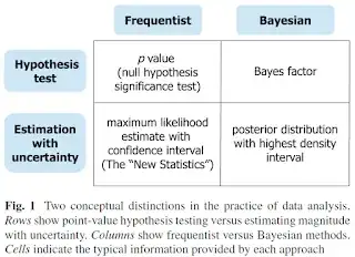
I come from a frequentist mindset by training, unfortunately. As such, I'm conditioned to interpret experimental results as either a) reject some null hypothesis, or b) fail to reject it, all based on a 95% level of confidence. I wish to understand how to interpret the results of basic Bayesian analyses, specifically credible intervals. In lieu of a frequentist technique (i.e. Fisher's Exact Test), I present the following example with a Bayesian approach.

A survey of aliens on two planets were asked if they eat apple pie:

$$\begin{array}{rcc} & \text{Yes} & \text{No} & \text{Total}\\ \hline \text{Martians} & 16 & 36 & 52\\ \text{Venusians} & 9 & 34 & 43\\ \text{Total} & 25 & 70 & 95\\ \hline \end{array}$$

$\mathbf{Hypothesis}$

The statistical hypothesis I wish to investigate is whether the proportion of Martians who eat apple pie is greater than Venusians who also eat apple pie.

$\mathbf{Beta{-}Binomial\ Model}$

The observed data has a total of $n_1=52$ Martians and $y_1=16$ eat apple pie. Also, we have $n_2=43$ Venusians and $y_2=9$ eat apple pie.

Let $\theta_1 \in [0,1]$ be the proportion of Martian pie-eaters and $\theta_2 \in [0,1]$ be Venusian pie-eaters. We model the pie-eaters as binomials:

$y_1 \sim \text{Binom}(n_1,\theta_1)$ and

$y_2 \sim \text{Binom}(n_2,\theta_2)$ and

Assume simple uniform priors on the proportions, which we know are equivalent to $\text{Beta}(1,1)$ priors:

$\theta_1 \sim \text{Unif}(0,1)=\text{Beta}(1,1)$ and

$\theta_2 \sim \text{Unif}(0,1)=\text{Beta}(1,1)$.

The beta distribution is a conjugate prior to the binomial: the resulting posterior is also a beta distribution. Thus, we can we can analytically compute the posteriors:

$p(\theta_1\mid y_1,n_1)=\text{Beta}(\theta_1\mid y_1+1,n_1-y_1+1)$ and

$p(\theta_2\mid y_2,n_2)=\text{Beta}(\theta_2\mid y_2+1,n_2-y_2+1)$

We could try to compute the posterior density of $\delta=\theta_1-\theta_2$ by solving the integral

$p\left( {\delta\mid y,n} \right) = \int_{ - \infty }^\infty {{\rm{Beta}}} \left( {\theta\mid {y_1} + 1,{n_1} - {y_1} + 1} \right){\rm{Beta}}\left( {\theta - \delta\mid {y_2} + 1,{n_2} - {y_2} + 1} \right)d\theta$

and then evaluate

$\rm{Pr}[\delta>0$].

Instead, we will estimate the integral by simulation. Take $M$ samples from the joint posterior

$p(\theta_1,\theta_2\mid y_1,n_1,y_2,n_2)=p(\theta_1\mid y_1,n_1)\times p(\theta_2\mid y_2,n_2)$,

which we express as

$(\theta_1^{(1)}, \theta_2^{(1)}), (\theta_1^{(2)}, \theta_2^{(2)}), (\theta_1^{(3)}, \theta_2^{(3)}),..., (\theta_1^{(M)}, \theta_2^{(M)})$

and compute the Monte-Carlo approximation

$\Pr \left[ {{\theta _1} > {\theta _2}} \right] \approx \frac{1}{M}\sum\nolimits_{m = 1}^M \mathbb{I} \left( {\theta _1^{\left( m \right)} > \theta _2^{\left( m \right)}} \right)$.

where $\mathbb{I}()$ is the indicator function which takes on the value 1 if its property is true and 0 if false.

All of that to say, we will estimate the probability that $\theta_1$ is greater than $\theta_2$ by the proportion of samples $m \in M$ where $\theta_1^{(m)}> \theta_2^{(m)}$.

$\mathbf{R\ code}$

### DATA
n1 = 52 # total number of Martians in the survey
y1 = 16 # number of Martians who eat apple pie
n2 = 43 # number of Venusians in the survey
y2 = 9  # number of Venusians who eat apple pie

### SIMULATION
R <- 100000 # number of simulations
theta1 <- rbeta(R, y1 + 1, (n1 - y1) + 1)
theta2 <- rbeta(R, y2 + 1, (n2 - y2) + 1)
diff <- theta1 - theta2  # simulated differences

quantiles <- quantile(diff,c(0.005,0.025,0.5,0.975,0.995))
print("Quantiles:")
quantiles

print("The probability that Martians eat apple pie to a greater extent compared to Venusians is:")
mean(theta1 > theta2)
print("The mean difference (theta1, theta2) is:")
mean(theta1 - theta2)
print("The median difference (theta1, theta2) is:")
median(theta1 - theta2)

### 95% CREDIBLE INTERVALS
# theta1
theta1ci <- quantile(theta1, c(0.025, 0.975))
theta1ci
# theta2
theta2ci <- quantile(theta2, c(0.025, 0.975))
theta2ci

### Comparison to specific computed instances of the beta distribution
### 95% Bayesian probability interval estimate
### See the following post for inspiration:
### https://math.stackexchange.com/questions/2704347/bayesian-confidence-interval-estimate-of-theta
# Martians
qbeta(c(.025,.975), 17, 37)
# Venusians
qbeta(c(.025,.975), 10, 35)

# VISULIZATION
# library(Cairo)
# CairoPDF(file = "bayes-contingency-cairo.pdf", family = "Helvetica")
plot(density(diff),
     xlab = "theta1 - theta2",
     ylab = "p(theta1 - theta2 | y, n)",
     main = "Applie Pie Consumption: \nPosterior Simulation of Martians vs. Venusians",
     ylim = c(0, 5),
     frame.plot = FALSE, cex.lab = 1.5, lwd = 3, yaxt = "no")
abline(v = quantiles[2], col = "blue")
abline(v = quantiles[4], col = "blue")
# dev.off()

$\mathbf{The\ Big\ Questions}$

After running the sumulation, we see that the credible intervals of Martians $\theta_1:[0.1988685, 0.4432125]$ and Venusians $\theta_2:[0.1139820, 0.3532699]$ overlap. In frequentist statistics, "confidence" intervals which overlap indicate non-significance.

1) How would I interpret these "credible" intervals from a Bayesian perspective?

2) There is an 85.4% chance that a higher prevalence of apple pie eating exists amongst Marians compared to Venusians. Although this percentage is not greater than 95% a la frequentist interpretation, how would one explain that this result is "significant"? Or, perhaps this finding is not worthy of further consideration since it is <95%?

Answer 1

In contrast to a frequentist viewpoint, a Bayesian viewpoint--to put it rather loosely--regards the observed data as fixed truths and the parameters of the underlying distribution to be random, whose variability from experiment to experiment is subject to the collection of more data. This turns the notion of a frequentist confidence interval on its head: a Bayesian's credible interval is a statement about the posterior probability of the parameter being in some subset of the parameter space. Your particular credible interval is constructed by finding the quantiles such that the tails of the posterior distribution are equiprobable, but this, like any other such interval extracted from the posterior distribution, is in some sense a crude statement about the parameter given the data, since such an interval does not tell us whether the posterior likelihood skews to one end of the interval or the other. Rather, it simply asserts that the probability of the parameter being in that interval is $0.95$. But as implied, such an interval is not unique among all intervals satisfying this property. There is no intrinsic reason why such an interval should be constructed with equiprobable tails.

As for the probability of one parameter being larger than the other, the pure Bayesian would probably avoid the "statistical significance" language of frequentists, because he or she would assert that $85.4\%$ captures the direct probability that the first proportion is higher than the second, and thus is a reflection of the strength of the difference between the two groups. But if we were to twist the purist's arm and use frequentist language, it is akin to the complement of the Type I error; thus the evidentiary bar does in fact need to be quite high in order to make the "assertion" that $\theta_1 > \theta_2$. But again, these are random variables, as evidenced by their posterior distributions. So unlike the frequentist's viewpoint, there is no such thing as categorically saying that $\theta_1 > \theta_2$ always. What you'd be saying if $\Pr[\theta_1 > \theta_2] \ge 0.95$ is literally that; the probability that the first rate exceeds the second is at least $0.95$ (given the data). The Bayesian can assign probabilities to such statements whereas a frequentist would balk, but the frequentist can assign probabilities to being right or wrong about some underlying, fixed, true state of reality, whereas the Bayesian cannot, because that reality is not fixed to him or her.

Answer 2

To see an explanation of frequentist and Bayesian approaches side by side, along with interpretations of credible intervals and confidence intervals, see this article:

Kruschke, J. K. (disclosure: that's me) and Liddell, T. M. (2018b). The Bayesian New Statistics: Hypothesis testing, estimation, meta-analysis, and power analysis from a Bayesian perspective. Psychonomic Bulletin & Review, 25, 178-206. https://link.springer.com/article/10.3758/s13423-016-1221-4

The figure below is the framework of the article. Notice that confidence and credilbe intervals show up in the lower row.