Extract data of 3D graph rendered in 2D

Question

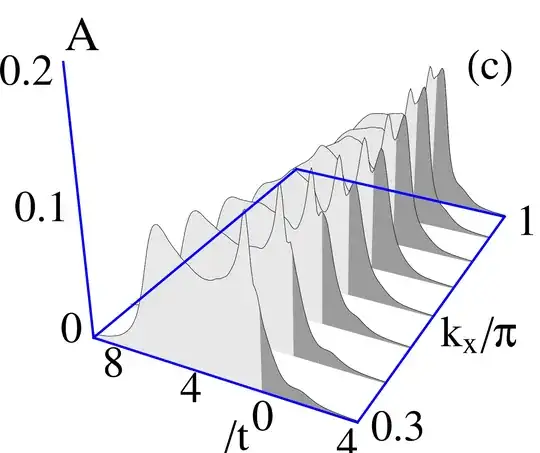
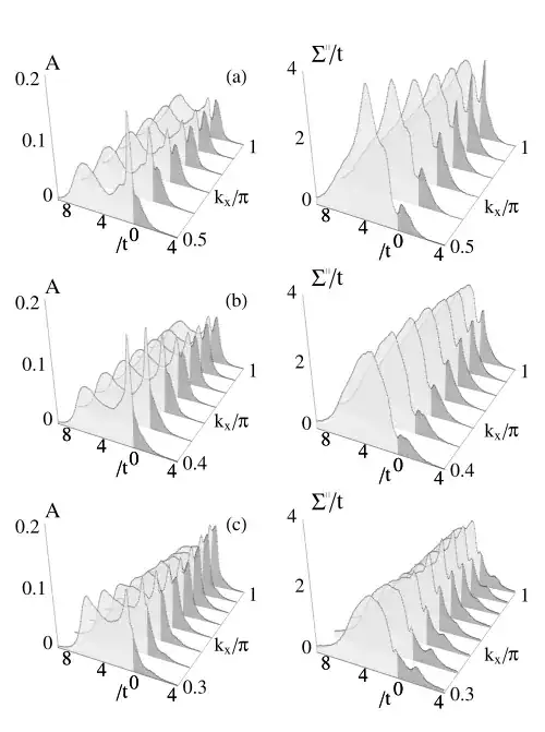
I have a 2D pdf of some 3D graphs from which I would like to extract the data (I have the authors permission, original data has since been lost). The graphs in question look like:

Focusing in on the bottom left graph, I can find the lines defining the axes like:

It seems like it would be quite simple to find a transformation which, when applied to a graph, would "straighten" it out so that the $x$ and $y$-axes correspond to vertical and horizontal positions on my screen. However I am really struggling to figure out what this transformation is. I guess I have a couple of questions

1. Do the blue lines in my second image provide enough information to define a transformation that will allow me view the graph "head-on"? (I feel like this is likely no?)
2. How would I go about finding such a transformation? What information would be needed? a. I've been reading about the Perspective-n-Point Method but am hoping there's an easier way before going further down that rabbit hole (I know next to nothing about computer vision).
   b. I followed the thread here How do I reverse-project 2D points into 3D? and was able to use a Monte-Carlo method to find a projection matrix - but that doesn't seem to help as it is a transformation from 3D to 2D instead of the reverse and it also seems like overkill.

Any help is highly appreciated, thanks!

UPDATE

This is the perspective issue I was trying to refer to in my comment below, thanks!

Answer 1

Andrei was correct about needing to do each curve separately, but the transformation he gave was slightly too simple so I am writing this answer share what I eventually ended up doing for those who come across this in the future.

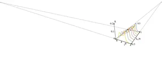
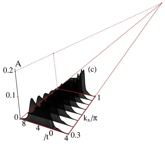
As shown in the update, the graphs are drawn with perspective. Turns out they are drawn with three point perspective which means the three vanishing points must be reconstructed. Two of the vanishing points are trivially defined by the axes:

We'll call them $vp_t$ and $vp_k$ from left to right.

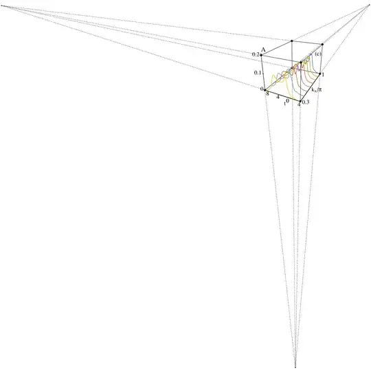
For the last vanishing point, $vp_A$, we only have a single $A$-axis so we need more information. Luckily projective geometry tells us that the cross ratio of four collinear points is invariant under projection. Along the $A$-axis we have 4 collinear points namely $p_0,p_{0.1},p_{0.2},$ and $vp_A$. Using the fact that the vanishing point is infinitely far away in "real space", this gives us the relation $$ \frac{|p_{0.2}-p_0||vp_A-p_{0.1}|}{|p_{0.1}-p_0||vp_A-p_{0.2}|}=\frac{0.2}{0.1}=2 $$ This expression combined with the equation for the line defining the $A$-axis uniquely determines the last vanishing point. With this third vanishing point, we can reconstruct the full cube containing our plots in projected space (2D) by finding the intersections of the relevant lines.

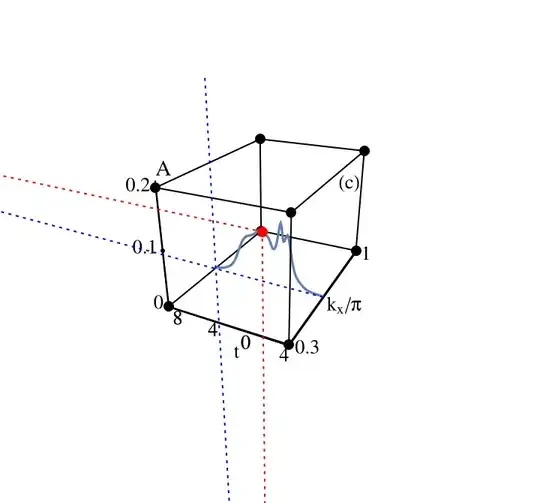
Armed with this box and the vanishing points the 3D data can be recovered by constructing the proper $A$-axis using $vp_A$ and $t$-axis using $vp_t$ then finding the intersection of these axes with the lines connecting the data point with the vanishing points. The data is finally extracted using the invariant cross-ratio above.

Answer 2

The trick is to do 2D transforms instead. I will explain for the last figure, but everything else is the same.

1. You digitize each curve separately.
2. You find the corresponding $k_x$ value by looking at the ratio of distances from the bottom corner to the points on that axis. It should be obvious that they increase by $0.1$. For example, you can get the bottom corner as $(x_B,y_B)$ and the right corner as $(x_R,y_R)$, and the last point for second curve is at $(x_{2R},y_{2R})$. Then you have $$\frac{x_{2R}-x_B}{x_R-x_B}=\frac{y_{2R}-y_B}{y_R-y_B}=\frac{k_x-0.3}{1-0.3}$$ To minimize errors, choose to find $k_x$ from the equation with the largest denominator. The way I see the figure, it looks like $y$ axis. That way uncertainties in reading $y_{2R}$ value will be divided by a bigger number.
3. Translate the vertical axis to one point of the curve, say to $(x_{2L},y_{2L})$. I am interested in the top point of the vertical axis. If the original was $(x_A,y_A)$, the translated point will be $(x_A',y_A')=(x_A+x_{2L}-x_L,y_A+y_{2L}-y_L)$ Then the transformation is given by $$\begin{pmatrix}t+8\\A\end{pmatrix}=M\begin{pmatrix}x-x_{2L}\\y-y_{2L}\end{pmatrix}$$ Here $M$ is a $2\times2$ matrix. To get the coefficients of the matrix, you know that you transform $(x_{2R},y_{2R}$ into $(4+8,0)$, and you transform $(x_A',y_A')$ into $(-8+8,0.2)$
4. Use the rest of the points in the digitized curve and the above transformation to get the "original" data.
5. Repeat for all curves

The procedure is not that difficult, but the trick is to consider each curve separately.

Answer 3

[Too long for a comment, so adding this as an answer to supplement yours.]

Once you’ve gotten the bounding “cube” for a graph set, I think you can save yourself quite a bit of work by computing a rectifying homography for each slice instead of painstakingly working out intersections and cross-ratios. For each slice, find the corners—the points at which the plane of the slice intersects the bounding cube—and then compute the mapping from this quadrilateral to an appropriately-sized rectangle using the method in this answer. For each graph, the $B$ matrix for this construction is constant. E.g., for the bottom left graph, the destination rectangle is $[-8,4]\times[0,0.2]$, which yields $$B = \begin{bmatrix}8&-8&4\\0&0.2&0\\-1&1&1\end{bmatrix}.$$ For the front slice of this graph (making my own guess at where the 0.1 point on the A axis lies), the homography matrix works out to be $$\left[ \begin{array}{ccc} 0.0119905 & 0.000455823 & -10.0139 \\ 0.0000677027 & 0.000210969 & -0.0960643 \\ 0.000150268 & 0.000123509 & 0.70175 \\ \end{array} \right].$$ Applying this matrix to points on the image of the front graph slice and dehomogenizing will recover their original coordinates. To illustrate, applying this transformation, combined with some scaling to make the destination rectangle a square, to the image of the graph produces the following rectified image:

For the other slices, you would need to compute the corresponding quadrilateral corners and homography.

To take a somewhat different approach, each graph contains enough known/measurable point pairs for you to recover the camera matrix $P$. (Indeed, it appears that they all basically use the same projection, so you could combine data from all of the graphs to sharpen up the estimate.) You can find methods for doing this in any standard reference on computer vision such as Hartley and Zisserman’s Multiple View Geometry In Computer Vision. Since you’ve computed/estimated the world axis vanishing points, you can use them as additional constraints on $P$: its first three columns are these image points. The last column of $P$ is the image of the world origin, which unfortunately can’t be measured directly in these graphs. So, $P$ will be of the form $$\begin{bmatrix}\lambda \mathbf v_X & \mu \mathbf v_Y & \tau \mathbf v_Z & \mathbf o\end{bmatrix}.$$ The last coordinate of $\mathbf o$ can be fixed at $1$, so there are 5 unknowns to be determined from known world-image point pairs.

Decomposing $P$ as $[M\mid\mathbf p_4]$, a point $\mathbf x$ in the image back-projects to the ray (in inhomogeneous Cartesian coordinates) $\tilde{\mathbf X}(\mu) = M^{-1}(\mu\mathbf x-\mathbf p_4)$. Rectifying each graph slice is then just a matter of intersecting this ray with the plane that represents the slice. These planes are all parallel to a coordinate plane, so the required computation is particularly simple.