2

I'm reading Hassani's Mathematical Methods book specifically the chapter on Integral Transforms. He derives the fourier transform starting with the concept that the fourier transform has a kernel of the form $e^{itx}$, everything goes well until he stated on the bottom of page 694,

"In other words, as $n$ changes by one unit, $k_n$ changes only slightly. This suggests that the terms in the sum in Equation (29.2) can be lumped together in $j$ intervals of width $\Delta n_j$"

That means as $\Lambda \rightarrow \infty $, $k_n \rightarrow 0$, so becomes almost continuous. The sentence "This suggests that the terms in the sum in Equation (29.2) can be lumped together in $j$ intervals of width $\Delta n_j$" is what I don't understand. Can anyone clarify what he meant?

1

2

3

  • I always hated argument like this and never found a book that present this claim rigorously. You can find that argument in nearly all introductory books on Fourier series and transform, and the "justication" is always a hand waving argument full of "we can guess that it is a good idea to take...", "we can expect that it is a good approximation...". Probably there's some value behind these crappy arguments, at least at the level of intuition, but I always thought that this is not the manner to present that result and that there's some way to prove a theorem that states that claim rigorously. – Bob Jul 29 '18 at 10:25
  • 1
    The rigour required to do Fourier analysis from start you would basically need a course in measure theory and functional analysis. But at the time when most (engineering) people learn practical Fourier methods they are nowhere near the mathematical maturity to digest the theory required for that. Just try to remember what annoyed you when you took the course and revisit it later on 1, 2, 5 or maybe 10 years. – mathreadler Jul 29 '18 at 11:15
  • Brown and Churchill has a good intuitive derivation of this type. The original argument of this type was given by Fourier. There was no other intuitive or direct way to obtain the Fourier transform and its inverse given by anyone for many decades after Fourier. So arguments of this type remain part of the folklore of the subject. They're great for thinking about how one might obtain the Fourier integral expansion from a limited of the discrete case on an interval, but I'm not aware of anyone making such arguments completely rigorous. – Disintegrating By Parts Jul 29 '18 at 16:02
  • @DisintegratingByParts Do Brown and Churchill discuss in detail fourier transforms? Based on the scan that I did it seems that they just leave it in the exercises. Also, if it is possible for someone to decipher what Hassani stated then it would be better. – mathemania Jul 29 '18 at 16:50
  • @mathemania here you can find my attempt to make the argument sensible: https://math.stackexchange.com/questions/2866510/filling-gaps-in-a-proof-of-fourier-inversion-formula – Bob Jul 30 '18 at 00:04
  • @mathemania : 51 : The Fourier Integral Formula in Fourier Series and Boundary Value Problems. They note that the derivation is not rigorous, but it is very compelling the way they present it as a passage from the finite to the infinite interval. – Disintegrating By Parts Jul 30 '18 at 22:00
  • @mathemania see the answer by David Ullrich to this question: https://math.stackexchange.com/questions/2872279/derive-fourier-transform-by-analogy-to-fourier-series – Bob Aug 05 '18 at 16:53

3 Answers3

2

"The terms in the sum can be lumped together" means that it can be possible to sum every $\Delta n_j$ consecutive terms (the resulting sum can be called lumped term) and then consider the series of such lumped terms as equivalent to the original series. In building such a lumped term some approximation can be made of the kind here illustrated. Fourier Transform

In the first diagram I plotted as an example the sequence $$\frac{1}{\sqrt{L+\Lambda}}f_{\Lambda, n}e^{2i\pi nx/(L+\Lambda)}$$ on $36$ points only, at $x=1$, with the hypotheses that $L+\Lambda=1$ and $f_{\Lambda, n}\equiv 1$.

Supposing to lump together terms every $\Delta n_j = 3$, the corresponding piece of sequence that results is displayed in the second diagram. You see that for instance the three consecutive red terms (all with unit modulus) sum up to a term whose modulus is a bit less than $3$.

This lumped term can be substituted for by an approximated lumped term given by $\Delta n_j$ times one of the consecutive terms to be lumped as if all such consecutive terms had the same phase. In the third diagram, such an approximation is displayed, where the approximated lumped term is taken as three times the central term of the consecutive terms to be lumped.

Note that such an approximation can be affected heavely by $f_{\Lambda, n}$ that I've been considering constant in the diagrams. If it takes values too different the lumped terms could no longer be approximated by one of the original terms multiplied by the number of consecutive terms, because such terms would have very different moduli and phases. But this is not a problem because whatever is the level of approximation you want there will always be a real value such that, whatever is $\Lambda$ greater than this value, that level of approximation is attained (as you can see by $(29.3)$).

trying
  • 4,756
  • 1
  • 13
  • 23
  • Certainly you do make a point but based on what I think is it not that because as $n$ changes by one unit $k_n$ changes only slightly and this in turn makes each term to vary only slightly with each other therefore this will transition to the concept of limits where if $\Delta n$ is infinitesimal then $k_n$ would be even smaller hence the function can be continuous if we change the sum to an integral wherein we change $\Delta n$ to $dn$. Correct me if I'm wrong. – mathemania Aug 06 '18 at 05:19
  • The bigger the $\Lambda$, the less consecutive terms vary w.r.t. each other (where by term is meant $f_{\Lambda, n}e^{2i\pi nx/(L+\Lambda)}$ in $(29.2)$ and "consecutive terms" means terms with $n$'s on a small integer interval). This is because the two factors of these terms have separately this same behaviour. In particular $e^{2i\pi nx/(L+\Lambda)}$ acts that way, as I have shown with the diagrams, while $f_{\Lambda, n}$ acts that way because of $(29.3)$. This behaviour justifies the use of approximated lumped terms and what follows from their use. – trying Aug 06 '18 at 07:51
  • Yes, so that means what I'm thinking is correct. – mathemania Aug 06 '18 at 13:10
0

It should be something like

This suggests that the terms in the sum in Equation (29.2) can be divided into pieces, where in each piece the quantity $k_n$ is constant. Denote the length of the $j$-th piece by $\Delta n_j$, and put $n=n_j$ throughout the $j$-th piece.

In other words, he is writing $$ \sum_{n}f_{\Lambda,n}e^{ik_nx}=\sum_j\sum_{n\in I_j}f_{\Lambda,n}e^{ik_nx}\approx\sum_jf_{\Lambda,n_j}e^{ik_{n_j}x}\Delta n_j $$ where $\{I_j\}$ is a disjoint decomposition of $\mathbb{Z}$ into intervals, $\Delta n_j=|I_j|$ is the number of elements of $I_j$, and $n_j\in I_j$ is an element of $I_j$ chosen by some rule.

timur
  • 16,599
0

I have a slightly different book that defines this differently. The motivation for the Fourier Transform can be seen from the following. This is from Richard Haberman - Applied Partial Differential Equations with Fourier Series and Boundary Problems

In solving boundary value problems on a finite interval $-L < x < L$ with periodic boundary conditions we can use the complex form of the Fourier Series

$$ \frac{f(x+)+f(x-)}{2}= \sum_{n=-\infty}^{\infty} c_{n}e^{\frac{-in \pi x}{L}}$$

Where $f(x)$ represents a linear combination of all the sinusoids that are periodic with period $2L$ then we have the Fourier coefficients as

$$c_{n} = \frac{1}{2L}\int_{-L}^{L} f(x)e^{\frac{-in \pi x}{L}}dx $$

now then we have $ -L < x < L $ as our region of integration. So we extend it to $ - \infty < x< \infty $

$$ \frac{f(x+)+f(x-)}{2}= \sum_{n=-\infty}^{\infty} \left[ \frac{1}{2L}\int_{-L}^{L} f(\bar{x})e^{\frac{-in \pi \bar{x}}{L}}d\bar{x} \right]e^{\frac{-in \pi x}{L}}$$

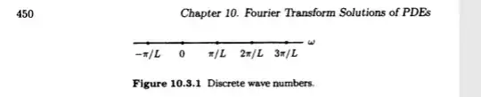
For periodic functions $ -L < x < L $ the number of waves $ \omega $ in a distance of $ 2 \pi $ are then

$$ \omega = \frac{n \pi}{L} = 2\pi \frac{n}{2L}$$

giving us the distance between waves $$ \Delta \omega = \frac{(n+1) \pi}{L} - \frac{n \pi}{L} = \frac{\pi}{L}$$

enter image description here

$$ \frac{f(x+)+f(x-)}{2}= \sum_{n=-\infty}^{\infty} \left[ \frac{\Delta \omega}{2\pi}\int_{-L}^{L} f(\bar{x})e^{i \omega \bar{x}}d\bar{x} \right]e^{-i \omega x}$$

Then the fourier transform here is as $ L \to \infty $. The values $ \omega $ are the square roots of the eigenvalues so they get closer and closer $ \Delta \omega \to 0$

$$ \frac{f(x+)+f(x-)}{2}= \frac{1}{2 \pi}\int_{-\infty}^{\infty} \left[ \int_{-\infty}^{\infty} f(\bar{x})e^{i \omega \bar{x}} \right]e^{-i \omega x} d\omega$$

Then the fourier transform is

$$F(\omega) = \frac{1}{2 \pi} \int_{-\infty}^{\infty} f(\bar{x}) e^{i \omega \bar{x}} d \bar{x} $$

The notation is that our interval $ - L < x < L$ has extended to infinity as you see. This is commonly what happens when you have some Riemann sum and take the discrete intervals and you let them go infinitly small.