Let's say I have a uniform distribution whose values range between $0$ and $1$. I now sample two values from this distribution and put them in the variables $x$ and $y$. I subsequently compute $x \cdot x$ and $x \cdot y$. Do the results of these follow the same distribution?
-
9Have you worked out the expectations of $x^2$ and $xy$? – kimchi lover Jan 27 '18 at 13:39
1 Answers
The short answer, suggested by @kimchilover, compares $E(X^2)$ and $E(XY).$ Because the expectations differ, $X^2$ and $XY$ can't have the same distribution.
First, $E(X^2) = \int_0^1 t^2 f_X(t)\,de = \int_0^1 t^2\, dt = \frac 1 3.$ Also, by independence, $E(XY) = E(X)E(Y) = \frac 1 4.$
However, this is a nice problem, and you may have something to learn by looking at it in more detail. It is not difficult to find the distribution of $V= X^2:$ For $0 < t < 1,$ we have the CDF $F_{V}(t) = P(X^2 \le t) = P(X \le \sqrt{t}) = \sqrt{t}.$ So the density function is $f_V(t) = \frac {1}{2\sqrt{t}}.$ Then a second way to find $E(X^2)$ is
$$E(X^2) = E(V) = \int_0^1 tf_V(t)\,dt = \int_0^1 \frac{1}{2}t^{1/2}\, dt = \frac 1 3.$$
Also, you could do a transformation to find the joint density of $W = XY$ and $X$ and 'integrate out' $X$ to get the marginal distribution of $W.$ Depending on the context of this problem, that derivation may be the main point of it, so I will leave it to you to finish the derivation. (Perhaps see this page.)
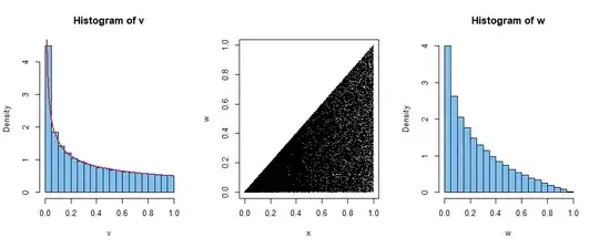
Note: Graphs based on random sample of $m = 50,000$ of $X$ and $Y$ illustrate some of the results. The first panel shows a histogram of $m$ values of $V$ along with the density function of $V \sim \mathsf{Beta}(.5, 1).$ The second panel suggests the bivariate distribution of $(U,W)$ and may help with the limits on the integral required to derive the marginal distribution of $W.$ The third panel shows a histogram of $m$ values of $W,$ roughly suggesting shape of the PDF of $W,$ but not showing it explicitly.
- 51,500
