The rational function $y/x$ is regular (i.e., defined) at every point on your curve $C$ other than the origin $P = (0,0)$, but at $P$ it is undefined. In order to get a function defined at the origin, we can blow up the point $P$, which will resolve the singularity at $P$.
The idea behind blowing up is the following. At a singular point $P$, there are multiple tangent lines. So we can replace that single point by several points, one for each tangent line, by adding another coordinate (a copy of $\mathbb{P}^1$) that keeps track of the slope of the tangent line. When $P = (0,0)$ is the origin, the slope is given by the function $y/x$, so our new coordinate $z$ will satisfy $z = y/x$, or $y = xz$ if we clear denominators. So really the blowup is (the closure of) the graph of the function $y/x$ on $C \setminus P$; see section 7.2 of Fulton's Algebraic Curves for details.
Your example is a bit confusing since the cuspidal cubic $y^2 = x^3$ has just one tangent line ($y = 0$) with multiplicity $2$ at the origin, so let's first consider the nodal cubic $y^2 = x^2(x + 1)$. Since its homogeneous term of lowest order is $y^2 - x^2 = (y - x)(y + x)$, then the nodal cubic has tangent lines $y = x$ and $y = -x$ at the origin. The function $y/x$ allows us to distinguish between the two branches of the curve. For points along the branch approximated by $y = x$ we have $y/x \approx 1$, and for those on the other branch, we will have $y/x \approx -1$.
So we will "pull apart" these branches by making a curve in $\mathbb{A}^2 \times \mathbb{P}^1$ whose $z$-coordinate is $y/x$. To find the equations for the blowup $\newcommand{\wt}{\widetilde} \wt{C}$, we simply substitute $y = xz$ in to the equations for $C$:
\begin{align*}
x^2(x+1) &= y^2 = x^2 z^2 \implies 0 = x^2(z^2 - (x+1)) = 0
\end{align*}
The factor of $x^2$ corresponds to the extra factor of $\mathbb{P}^1$ we introduced, while the other factor gives us the relation $x = z^2 - 1$. Since $y = xz$, we find the parametric curve
$$
\newcommand{\C}{\mathbb{C}}
\wt{C} = \{(z^2 - 1, z(z^2 - 1), z) : z \in \C\} \, .
$$
Below is the plot (made in SageMath) of the original curve, the blowup, and the points where it intersects the added copy of $\mathbb{P}^1$.
$\hspace{3cm}$ 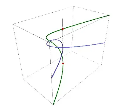
We can do the same thing in the case of the cuspidal cubic, obtaining the parametric curve
$$
\wt{C} = \{(z^2 , z^3, z) : z \in \C\}
$$
as shown in Zach Teitler's answer.
$\hspace{3cm}$ 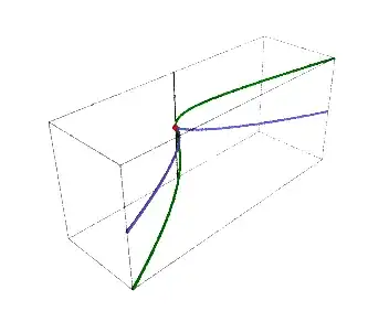
It's kind of hard to see what's going on from these still images, so it might be more illuminating to play with the interactive plots (made with SageMathCell) yourself: nodal cubic, cuspidal cubic.
The code for these plots is below.
# nodal cubic
var('t')
p1 = parametric_plot((t^2-1,t*(t^2-1),0), (t,-1.5,1.5), thickness = 2)
p2 = parametric_plot((t^2-1,t*(t^2-1),t), (t,-1.5,1.5), color = "green", thickness = 2)
p3 = parametric_plot((0,0,t), (t,-1.5,1.5), color = "black")
pts = point([(0,0,-1), (0,0,1)], color = "red", size = 5)
show(p1+p2+p3+pts)
# cuspidal cubic
var('t')
p1 = parametric_plot((t^2,t^3,0), (t,-1.5,1.5), thickness = 2)
p2 = parametric_plot((t^2,t^3,t), (t,-1.5,1.5), color = "green", thickness = 2)
p3 = parametric_plot((0,0,t), (t,-1.5,1.5), color = "black")
pts = point([(0,0,0)], color = "red", size = 5)
show(p1+p2+p3+pts)
This paper and this webpage have some great images, too.

