This is an answer for the 2-dimensional curl only. Hopefully one can turn it into a general argument for 3 dimensions.
Consider a perfect rotation of the plane around the origin, in which, at time $t$, a point $(x,y)$ is sent to
$$
R_t(x,y) =
\left[\matrix {\cos(\omega t) & -\sin(\omega t) \cr \sin(\omega t) & \hfill\cos(\omega t)}\right]
\left[\matrix {x \cr y }\right] =
\left[\matrix {x\cos(\omega t) -y \sin(\omega t) \cr x\sin(\omega t) + y\cos(\omega t)}\right].
$$
Observe that each point completes a full turn, namely $2\pi $ radians, as $t$ goes from zero to $2\pi /\omega $, so the angular velocity is
$$
\frac{\Delta \theta }{\Delta t} = \frac{2\pi }{2\pi /\omega } = \omega .
$$
The linear velocity vector at time zero of each point $(x, y)$ is given by
$$
\left.\frac d{dt}\right|_{\, t=0} R_t(x,y) =
\left[\matrix {-\omega x\sin(\omega t) -\omega y \cos(\omega t) \cr
\hfill \omega x\cos(\omega t) - \omega y\sin(\omega t)}\right]_{\, t=0} =
\left[\matrix {-\omega y \cr \hfill \omega x}\right],
$$
so the velocity vector field may be represented by
$$
F(x,y) = (-\omega y,\omega x) = \omega (-y,x).
$$
Given any point $(x, y)$ in the plane, let $C$ be the circle about the origin passing thru $(x,y)$, and observe that
the unit vector $\vec t\ $ tangent to $C$ at $(x,y)$ is given by
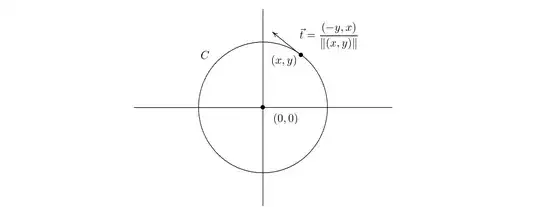
If we project $F(x,y)$ onto this vector (notice that these vectors are parallel, although in the more general situation
we are about to consider they might not be), we get the component of $F(x,y)$ that is causing a rotation around the origin, which is then given by
$$
\langle F(x,y),\vec t\ \rangle =
\left\langle (-\omega y,\omega x), \frac{(-y, x)}{\|(x, y)\|} \right\rangle =
\frac{\omega (y^2+x^2)}{\|(x, y)\|} =
\omega \|(x, y)\|.
$$
Consequently we may estimate the value of $\omega $ in terms of the vector field at any point $(x,y)$ by the simple formula
$$
\omega = \frac{\langle F(x,y),\vec t\ \rangle }{\|(x, y)\|}.
\tag 1
$$
If, instead of the origin, we consider a rotation about another point $(x_0, y_0)$, so that
$$
R_t(x,y) =
\left[\matrix {x_0 \cr y_0 }\right] +
\left[\matrix {\cos(\omega t) & -\sin(\omega t) \cr \sin(\omega t) & \hfill\cos(\omega t)}\right]
\left[\matrix {x-x_0 \cr y-y_0 }\right] =
\left[\matrix {x_0 + (x-x_0)\cos(\omega t) -(y-y_0) \sin(\omega t) \cr y_0 +(x-x_0)\sin(\omega t) + (y-y_0)\cos(\omega t)}\right],
$$
the corresponding velocity vector field would be given by
$$
F(x,y) = \omega (-y+y_0,x-x_0),
$$
while estimate (1) would be written as
$$
\omega = \frac{\langle F(x,y),\vec t\ \rangle }{\|(x-x_0, y-y_0)\|},
\tag 2
$$
where $\vec t$ is now given by
$$
\vec t = \frac{(-y+y_0, x-x_0)}{\|(x-x_0, y-y_0)\|}.
$$
Now suppose we are presented with an arbitrary vector field on the plane, say
$$
F(x,y) =\big (P(x,y),Q(x,y)\big ),
$$
and we want to estimate how much it rotates about a point $(x_0, y_0)$.
Notice that (2) would no longer be of much use since the field might perhaps be constant, meaning that all points are moving along
the same direction, without any rotation taking place, and still the RHS of (2) could yield a meaningless big value of $\omega $.
If you hold a child by the hand when strolling, you might not know whether they are walking straight or dancing around. But if the parents each hold one hand, it is much easier to tell!
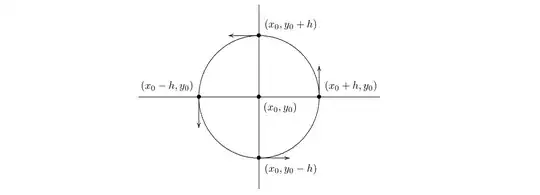
To account for this, let us choose many points, rather than just one, and average the outcomes of (2) for these
points. A reasonable choice would be four points, to the right, to the left, above and below the point $(x_0,y_0)$
under consideration.
Fixing a parameter $h>0$, let us then consider the following four points
$$
\matrix{
(x_1, y_1) &=& (x_0+h, y_0) & \quad \text{(right)} \cr
(x_2, y_2) &=& (x_0-h, y_0) & \quad \text{(left)} \cr
(x_3, y_3) &=& (x_0, y_0+h) & \quad \text{(above)} \cr
(x_4, y_4) &=& (x_0, y_0-h) & \quad \text{(below)}
}
$$
Regarding $(x_1, y_1)$, for example, we would have
$$
\vec t = (0, 1),
$$
so
$$
\omega _1 =
\frac{\langle F(x_0+h,y_0),(0, 1)\rangle }{\|(h, 0)\|} =
\frac{Q(x_0+h,y_0)}h.
$$
Averaging the four angular velocity estimates $\omega _1$, $\omega _2$, $\omega _3$, and $\omega _4$, we get
$$
\frac {\omega _1+ \omega _2 +\omega _3 + \omega _4}4 =
\frac { Q(x_0+h,y_0) - Q(x_0-h,y_0) - P(x_0,y_0+h) - P(x_0,y_0-h)}{4h}.
$$
In order to compute the infinitesimal angular velocity at $(x_0,y_0)$ we take the limit as $h\to 0$, which we may
compute using L'Hopital rule, leading up to
$$
\lim_{h\to 0_+} \frac {\omega _1+ \omega _2 +\omega _3 + \omega _4}4 =
\frac 1 4 \left(\frac {\partial Q}{\partial x}(x_0,y_0) + \frac {\partial Q}{\partial x}(x_0,y_0)
- \frac {\partial P}{\partial y}(x_0,y_0) - \frac {\partial P}{\partial y}(x_0,y_0)\right) = $$$$ =
\frac 1 2 \left(\frac {\partial Q}{\partial x}(x_0,y_0) - \frac {\partial P}{\partial y}(x_0,y_0)\right) =
\frac 1 2 \text{ curl }F(x_0,y_0).
$$
Although I was brought up as a mathematician, I was always much irritated when professors introduced new
concepts named after physically significant phenomenon without explaining in depht where the motivation for the
name came from. Some of my first
disapointments occured precisely when I was first confronted with the notions of gradient, divergent and curl.
Searching for an explanation does not always bring about any light and this in fact makes me suspect that lots of grown ups
have been force fed these concepts to the point that they eventually seem natural, after which one no longer feels the need for any further explanations.
Take the MIT course mentioned in @symplectomorphic's answer, for example.
There, Green's Theorem is used to explain that the 2-dimensional curl is related to the angular velocity of a small
paddle wheel. Could Green's Theorem historically have come before the notion of curl?
To me this makes no sense as it might give students the impression that Green first obtained his formula out of the blue and then, as an
afterthought, realized that his Theorem could be used to deduce that the curl represents the rotation of a vector field.

