The least squares fit is the best fit of the model to the data in the $2-$norm. This in no way implies the model is appropriate.
To quantify the quality of the fit, we must resolve the error in the fit parameters. After doing so, we can present graphical measures of quality.
Error propagation
The method of least squares is a powerful tool which not only estimates the fit parameters, but also provides quantitative assessment of the quality of parameters. The quantitative assessment is too often ignored.
One way to phrase your question is to ask? How can we tell if our solution is
$$
y(x) = 1.0000\pm 0.0002 + \left( 2.0000 \pm 0.0002 \right)x,
$$
or
$$
y(x) = 1.0 \pm 0.8 + \left( 2.0 \pm 0.7 \right)x?
$$
Are the measurements made with a yard stick or a \$$1000$ micrometer? The quality of the measurement propagates through the computation in a formal manner.
Example

The data, listed below, are from Bevington's book $\S$ $6.1$ which describes temperature measurements for a bar of material abutted by constant temperature heat baths as depicted above.
The measurements are a sequence of $m=9$ measurements of the form $$\left\{ x_{k}, T_{k} \right\}.$$
The model posited in a linear function
$$
T(x) = a_{0} + a_{1} x
$$
Least squares problem
Define the residual data vector as the difference between the measurement and the prediction:
$$
r_{k} = T_{k} - T\left( x_{k} \right)
$$
The least squares problem minimizes the total error $r^{2} = r\cdot r$.
Data
The measurement locations, $x_{k}$, are marked on the bottom of the bar shown above. The measured temperature, $T_{k}$, is compared to the predicted $T(x_{k})$
$$
\begin{array}{rrll}
x_{k} & T_{k} & \quad T(x_{k}) & \qquad r_{k} \\\hline
1 & 15.6 & 14.2222 & -1.37778 \\
2 & 17.5 & 23.6306 & \phantom{-}6.13056 \\
3 & 36.6 & 33.0389 & -3.56111 \\
4 & 43.8 & 42.4472 & -1.35278 \\
5 & 58.2 & 51.8556 & -6.34444 \\
6 & 61.6 & 61.2639 & -0.336111 \\
7 & 64.2 & 70.6722 & \phantom{-}6.47222 \\
8 & 70.4 & 80.0806 & \phantom{-}9.68056 \\
9 & 98.8 & 89.4889 & -9.31111 \\
\end{array}
$$
Linear System
The linear system relates the solution parameters of intercept $a_{0}$ and slope $a_{1}$ to the measurements:
\begin{equation}
\begin{array}{cccc}
\mathbf{A} &a &= &T\\
\begin{bmatrix}
1 & 1 \\ 1 & 2 \\ 1 & 3 \\ 1 & 4 \\ 1 & 5 \\ 1 & 6 \\ 1 & 7 \\ 1 & 8 \\ 1 & 9
\end{bmatrix}
& \begin{bmatrix}
a_{0} \\ a_{1}
\end{bmatrix}
&=&
\begin{bmatrix}
15.6 \\ 17.5 \\ 36.6 \\ 43.8 \\ 58.2 \\ 61.6 \\ 64.2 \\ 70.4 \\ 98.8
\end{bmatrix}
\end{array}
\end{equation}
Normal equations
The normal equations will provide not only the solution parameters, but also the curvature matrix, critical for the error estimates.
\begin{equation}
\begin{array}{cccc}
%
\mathbf{A}^{*} \mathbf{A} &a &= &\mathbf{A}^{*} T\\
%
% A*A
\begin{bmatrix}
9 & 45 \\
45 & 285 \\
\end{bmatrix}
% a
& \begin{bmatrix}
a_{0} \\ a_{1}
\end{bmatrix}
&=&\frac{1}{10}
\begin{bmatrix}
4667 \\ 28980
\end{bmatrix}
\end{array}
\end{equation}
Least squares solution
The particular solution to the least squares problem is
$$
\begin{bmatrix}
a_{0} \\ a_{1}
\end{bmatrix}_{LS}
=
\left( \mathbf{A}^{*} \mathbf{A} \right)^{-1}\mathbf{A}^{*} T
\begin{bmatrix}
4.81389 \\
9.40833
\end{bmatrix}_{LS}
$$
How many of these digits are significant? This is another way to phrase your question.
Error propagation
Bevington's $\S 6-5$ is a succinct explanation of error propagation. Measurements are inexact, therefore results will be inexact. There is a calculus for propagating errors through the computation. The beauty of the method of least squares is that the error in the solution parameters can be expressed in terms of the error in the data.
The computation chain begins with an estimate of the parent standard deviation which is based upon the total error:
$$
s^{2} \approx \frac{r^{2}} {m-n}.
$$
The parameter $m$ is the number of measurements, $n$ is the number of free parameters, here $(m,n)=(9,2)$.
Error contributions for individual parameters are harvested from the diagonal elements of the matrix inverse:
$$
\alpha = \left( \mathbf{A}^{*} \mathbf{A} \right)^{-1}
$$
Older terminology calls $\alpha$ the curvature matrix.
Let
$$
\Delta = \det \left( \mathbf{A}^{*} \mathbf{A} \right)
$$
$$
\begin{align}
\epsilon_{0}^{2} &= \frac{r^{\mathrm{T}}r}{\Delta\left( m-n \right)} \sum x_{k}^{2} \\
\epsilon_{1}^{2} &= \frac{r^{\mathrm{T}}r}{\Delta\left(m-n \right)} \sum 1 \\
\end{align}
$$
Final result
The errors indicate the significant digits.
$$
\begin{bmatrix}
a_{0} \\ a_{1}
\end{bmatrix}_{LS}
=
\begin{bmatrix}
4.8 \pm 4.9 \\
9.41 \pm 0.86
\end{bmatrix}_{LS}
$$
For validation, these are intermediate values: $\Delta=540$, $r^{2}\approx317$.
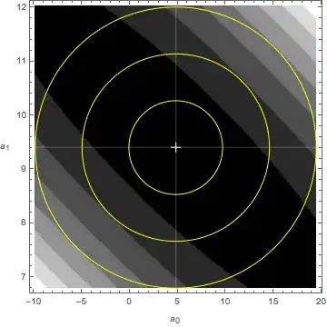
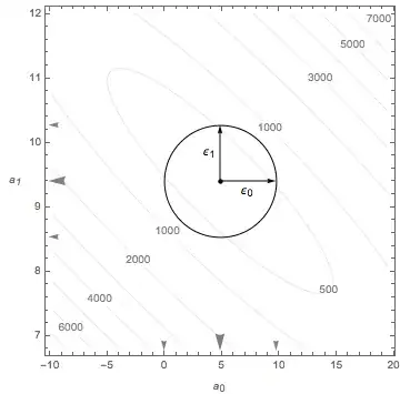
Pictures
The target of minimization, the merit function $M(a)$, is plotted below. The minimum is marked and surround by yellow rings representing 1, 2, and 3 $\epsilon$ values.
$$
M \left( a_{0}, a_{1} \right) = \sum_{k=1}^{m} \left( T_{k} - a_{0} -
a_{1}x_{k}\right)^{2}
$$
Another view shows the first error ellipse only.
The uncertainty parameters describe the width of the Gaussian distribution. Tighter measurements = better quality = skinnier peak. Below, the distributions for both parameters are plotted against the same scale. Certainly the intercept parameter is a noisier measurement.

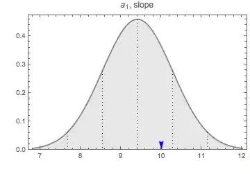
For these data, the expectations is that the intercept is $a_{0}=0$ and the slope $a_{1}=10$. Is this consistent with the result? The blue arrowheads in the above figures show the ideal points.
Finally, look at two different ways to envision the statistical variance. Using the Gaussian widths above, two hundred different sets of solution parameters (black dots) were plotted against the measurement (red cross). The rings represent 1, 2, and 3 standard deviations and provide a qualitative feel for how many points to expect in each band.

The last plot is a whiskers plot. It takes each of the 200 solutions and plots them against the data set. The white points are the ideal expectations.

Reference
Data Reduction and Error Analysis
Philip R. Bevington
McGraw-Hill, 1969 (1e)


