How to plot $N$ points on the surface of a $D$-dimensional sphere roughly equidistant apart?

Question

Let's say I have a $D$-dimensional sphere with a radius $R$. I want to plot $N$ number of points evenly distributed (equidistant apart from each other) on the surface of the sphere. It doesn't matter where those points are exactly, just that they are ROUGHLY equidistant from each other. How would I do this?

Answer 1

Firstly, I realize this question is $9$ years old; nonetheless, I have come up with a way to generate points roughly uniformly on the surface of a $D$-dimensional sphere.

Secondly, we aren't looking for equidistant points, only "neighbours" of each point will be equidistant from the original point, otherwise we would always have $N \le D+1$, and the points would land on the vertices of a $D$-dimensional tetrahedron.

What I assume we actually mean is "uniformity", meaning that the minimum distance between two points is maximal (and this minimum distance is taken on many many times, namely between neighbouring points).

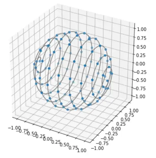
In $3$ dimensions, this can be achieved with the socalled Fibonacci-sphere, however, even though this "looks" impressive, the points aren't truly uniformly spaced. Here is the Fibonacci-sphere algorithm on the unit-sphere in Python (taken from this post on StackOverflow by user Fnord). I have generated $100$ points with it, and printed out the distances between each of the points.

def fibonacci_sphere(samples=100):
points = []
phi = math.pi * (3. - math.sqrt(5.))  # golden angle in radians

for i in range(samples):
    y = 1 - (i / float(samples - 1)) * 2  # y goes from 1 to -1
    radius = math.sqrt(1 - y * y)  # radius at y

    theta = phi * i  # golden angle increment

    x = math.cos(theta) * radius
    z = math.sin(theta) * radius

    points.append((x, y, z))

return points


def dist(u,v):
    return math.sqrt(sum([(u[i]-v[i])**2 for i in range(len(u))]))
points = fibonacci_sphere(100)
distances = [[dist(points[u],points[v]) for u in range(v)] for v in range(len(t))]
distances_flat = [item for sublist in distances for item in sublist]
sorted_distances = sorted(distances_flat)
sorted_distances

The result was the following list:

$$\begin{array}{l}0.20100756305184192,\\ 0.2010075630518425,\\ 0.2842676218074806,\\ 0.28426762180748066,\\ 0.320805901687651,\\ 0.3208059016876548,\\ 0.3298116166249696,\\ 0.32981161662497394,\\ 0.33090908965129245,\\ 0.3309090896512976,\\ 0.3330182810623833,\\ 0.3330182810623897,\\ 0.3331677084888959,\\ 0.3331677084888995,\\ 0.33368294298890966,\\ 0.33368294298891393,\\ 0.33392265293554585,\\ 0.3339226529355514,\\ 0.33512888128223783,\\ 0.33512888128224555\end{array}\\ \vdots$$

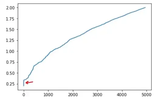
The minimum distance between each pair of points isn't actually taken on as many times as we would expect. However, if we were to plot these values, we can see that there is a significant jump at the start, meaning that only a few points are actually "somewhat close" to each other:

While this method is hard to reproduce in higher dimensions, I have found a different method with similarly good results, which I call the "spiral method". The idea is to map a straight line onto the surface of the sphere in a spiral method, then place equidistant points on the line:

Before I share the generating method, I will show the same sorted list, containing the distances between each pair of points:

$$\begin{array}{l}0.20100756305184192,\\ 0.2010075630518425,\\ 0.28212636061512686,\\ 0.28212636061512686,\\ 0.28421841394073166,\\ 0.2842184139407317,\\ 0.28426762180747983,\\ 0.28426762180748066,\\ 0.2857776209110349,\\ 0.28577762091103565,\\ 0.28826088539522315,\\ 0.28826088539522315,\\ 0.2890228024250095,\\ 0.2890228024250097,\\ 0.29109957918517715,\\ 0.29109957918517715,\\ 0.29378768027152646,\\ 0.2937876802715268,\\ 0.29424149806276\end{array}\\ \vdots$$

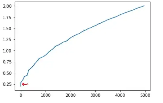
It's not significantly worse than the Fibonacci method, I'd say. Plotting these values gives:

There is a slightly shorter vertical section at the start, but importantly, the minimum distance between points is the exact same value, about $0.201$.

Now for the parametrization of the curve:

$$x(t) = t\\ y(t) = \sqrt{1-t^2}\cos\left(\left(1-\frac{1}{3}\sqrt{1-t^2}\right)\sqrt{N}ct\right)\\ z(t) = \sqrt{1-t^2}\sin\left(\left(1-\frac{1}{3}\sqrt{1-t^2}\right)\sqrt{N}ct\right)\\ t \in [-1,1]$$

where $c$ is a proportionality factor, namely the optimal $c$ in $3$ dimensions is

$$c = \pi$$

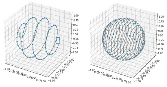
If we choose $c$ to be smaller, then there would be fewer revolutions around the sphere, and if $c$ was larger, then there would be more revolutions. In the following example, I set $c$ to be $\frac{\pi}{2}$ on the left, and $2\pi$ on the right. In both caes, there will be some points that are "too close" to each other:

To extend the problem into $4$ dimensions and higher, we will do the following:

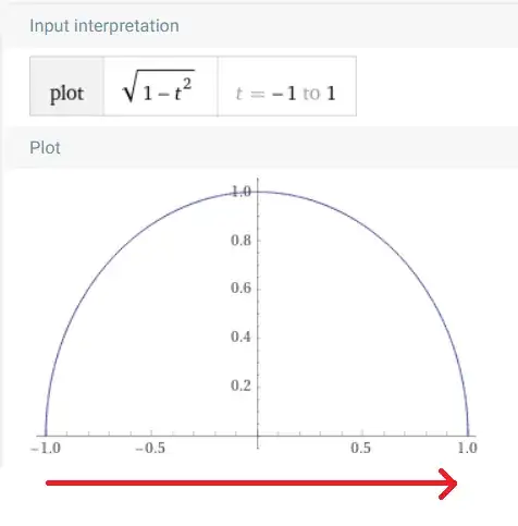
"$\sqrt{1-t^2}$ rule": Move the spiral along the new direction with the rate of $\sqrt{1-t^2}, t \in [-1,1]$.

This will clearly move the spiral homogeneously along the new direction, since the parametrization of the upper half of the circle in the new direction is $\sqrt{1-t^2}, t \in [-1,1]$. For those that are more visual, this is the "speed" at which we move the spiral with towards the new direction:

As you can see, this exactly describes the upper half of a circle.

However, $t$ isn't simply a linear factor in our case, it's instead the distance between the $z$ axis and each point of the spiral, namely

$$\sqrt{x(t)^2 + y(t)^2} =\\= \sqrt{t^2 + \sqrt{1-t^2}\cos\left(\left(1-\frac{1}{3}\sqrt{1-t^2}\right)\sqrt{N}ct\right)}$$

So using this in place of $t$, we can generate the $4$-dimensional spiral,

$$x(t) = t\\ y(t) = \sqrt{1-t^2}\cos\left(\left(1-\frac{1}{3}\sqrt{1-t^2}\right)\sqrt{N}ct\right)\\ z(t) = \sqrt{1-x(t)^2-y(t)^2}\cos\left(\left(1-\frac{1}{3}\sqrt{1-t^2}\right)\sqrt{N}ct\right)\\ w(t) = \sqrt{1-x(t)^2-y(t)^2}\sin\left(\left(1-\frac{1}{3}\sqrt{1-t^2}\right)\sqrt{N}ct\right)\\ t \in [-1,1]$$

However, there is a caveat. Even though we traced out the surface of the $4$-dimensional sphere, the spirals might not be correctly spaced from each other. So we have to recalculate / estimate the new $c$. We can do this using binary search, while optimizing the shortest distance between the generated points.

For $4$ dimensions, the best $c$ I was able to find using binary search was $c=4.8361682697$, however, I'm not sure how this relates to $\pi$ in the $3$-dimensional case. For this $c$, and $N=100$ points, the minimum distance between two points was $0.1879594048539$.

This gives us an algorithm for generating points in $D$ dimensions:

$1$. Input: $D \ge 3$: desired dimension; $N \ge 1$: desired number of points.

$2$. Define the following functions: $$x_1(t,c) := t\\ x_2(t,c) := \cos\left(\left(1-\frac{1}{3}\sqrt{1-t^2}\right)\sqrt{N}ct\right)$$

$3$. for $k=3,\dots,D$ do:

$$x_1(t,c) := x_1(t,c)\\ x_2(t,c) := x_2(t,c)\\ \vdots\\ x_{k-2}(t,c) := x_{k-2}(t,c)\\ x_{k-1}(t,c) := \sqrt{1-\sum_{i=1}^{k-2} x_i^2(t,c)} \cos\left(\left(1-\frac{1}{3}\sqrt{1-t^2}\right)\sqrt{N}ct\right)\\ x_{k}(t,c) := \sqrt{1-\sum_{i=1}^{k-2} x_i^2(t,c)} \sin\left(\left(1-\frac{1}{3}\sqrt{1-t^2}\right)\sqrt{N}ct\right)$$

$4$. Use binary search for $c$ to minimize $$\min_{c} \max_{i,j \in \{0,\dots,N-1\},\ i \ne j}(||p_i-p_j||_2^2)$$ where the $p_i$'s are the generated points, namely $$p_i = \left(x_1\left(\frac{2i}{N-1}-1,c\right),\dots,x_D\left(\frac{2i}{N-1}-1,c\right)\right)$$ $i = 0,\dots,N-1$. (This way, the $p_i$'s are uniformly spaced on $[-1,1]$.)

$5$. Output $p_0,\dots,p_{N-1}$ with the optimal $c$.

Where in step $3$, generate the curve for dimensions $k=3,4,\dots,D$, step by step by leaving the first $k-2$ arguments, and changing the last two arguments according the the $\sqrt{1-t^2}$ rule.

I'll leave the $5$D example here too, just to make sure everything is clear:

$$x(t) = t\\ y(t) = \sqrt{1-t^2}\cos\left(\left(1-\frac{1}{3}\sqrt{1-t^2}\right)\sqrt{N}ct\right)\\ z(t) = \sqrt{1-x(t)^2-y(t)^2}\cos\left(\left(1-\frac{1}{3}\sqrt{1-t^2}\right)\sqrt{N}ct\right)\\ w(t) =\\= \sqrt{1-x(t)^2-y(t)^2-z(t)^2}\cos\left(\left(1-\frac{1}{3}\sqrt{1-t^2}\right)\sqrt{N}ct\right)\\ v(t) =\\= \sqrt{1-x(t)^2-y(t)^2-z(t)^2}\sin\left(\left(1-\frac{1}{3}\sqrt{1-t^2}\right)\sqrt{N}ct\right)\\ t \in [-1,1]$$

Answer 2

If $N \le D + 1$ all points must be located on $N-1$ dimension equilateral triangle.

UPDATE

So, I thought today at this problem and invented method, contains following steps:

1. Generating $N$ random points on sphere $R$ (that is generating points with coordinates with Gaussian distribution).
2. Building Convex Hull (or triangulation on hypersphere even better) with generated on first step points. This step can be solved with MIConvexHull library if you familar with C#, similar library on your favorite language or your own code.
3. Using Genetic algorithm, Simulated annealing or another method of global optimization. This method then have to be applied to variance value of all edge lengths from convex hull from step 2.